9 Quantifying model uncertainty

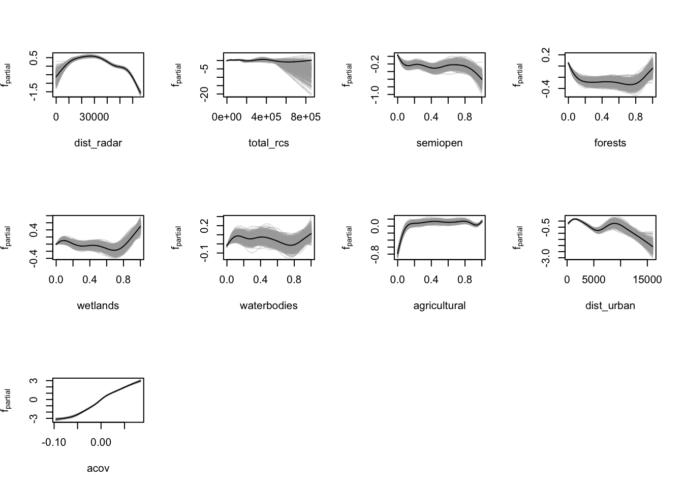
We use a boostrapping approach to quantify model uncertainty. Luckily, the mboost already contains the functions to do so. The partial dependence plots generated in the previous chapter visualise the marginal effect of certain predictors on the outcome log(VIR). We use a bootstrapping approach to quantify the model uncertainty.

9.1 Processing environment

library(parallel)
library(tibble)
library(dplyr)
library(tidyr)
library(patchwork)

9.2 Bootstrapped uncertainty analysis

Using the bootstrapping procedure provided in mboost, tweaked to our use case, we can derive uncertainty estimates from the trained model.

We make a few changes to the default functioning of the confint.mboost function.

1. We let bootstrap folds be determined outside of the function call, so they can be stored separately and processing can be parallellised more easily.
2. We include variable importance as variable to be bootstrapped, so uncertainty estimates around that value can be quantified too.
3. We calculate model predictions for a finer grid along the variables of interest (1000 values instead of 100).

9.2.1 Determine bootstrap folds

The folds contain indexes of datapoints that are resampled for each of the 1000 bootstrap iterations.

model <- readRDS("data/models/model_rac.RDS")
folds <- mboost::cv(model.weights(model), B = 1000)
saveRDS(folds, file = "data/models/confints/folds.RDS")

9.2.2 Running the bootstrapping procedure

It is very computationally intensive to execute the bootstrapping procedure, hence it is best executed manually tweaking settings to the local machine (memory, CPU cores, etc). See the R/mboost_uncertainty_analysis.R file for an example of how to do so. In this case I had 2-3 RStudio jobs running the script on a batch of the folds, which can be combined later on as results are stored in data/models/confints/. Execution took about 3 days.

source("R/mboost_uncertainty_analysis.R")

9.3 Recombine bootstrapped results

Having adjusted the bootstrapping procedure a bit, we now have to recombine the data so the R object matches the format mboost functions expect. Additionally, we will include the variable importance now as well.

n_confint_files <- length(Sys.glob("data/models/confints/modelci*"))
confint_files <- paste0("data/models/confints/modelci_", 2:n_confint_files, ".RDS")
cis <- lapply(confint_files, readRDS)
ci_boot_pred <- lapply(cis, function(x) x$boot_pred)
ci_varimp <- lapply(cis, function(x) x$varimp)

modelci <- readRDS("data/models/confints/modelci_1.RDS")
modelci$boot_pred[2:n_confint_files-1] <- ci_boot_pred
modelci$boot_pred[1] <- NULL
modelci$data <- cis[[1]]$data
modelci$varimp <- ci_varimp

saveRDS(modelci, file = "data/models/confints/final_modelci.RDS")

Let’s confirm it worked by plotting the bootstrapped confidence intervals.

vars <- c("dist_radar", "total_rcs", "semiopen", "forests", "wetlands", "waterbodies", "agricultural", "dist_urban", "acov")
par(mfrow = c(3, 4))
lapply(vars, function(x) plot(modelci, which = x, raw = TRUE))

## [[1]]
## NULL
## 
## [[2]]
## NULL
## 
## [[3]]
## NULL
## 
## [[4]]
## NULL
## 
## [[5]]
## NULL
## 
## [[6]]
## NULL
## 
## [[7]]
## NULL
## 
## [[8]]
## NULL
## 
## [[9]]
## NULL

Voilà, that seems to have done the trick.