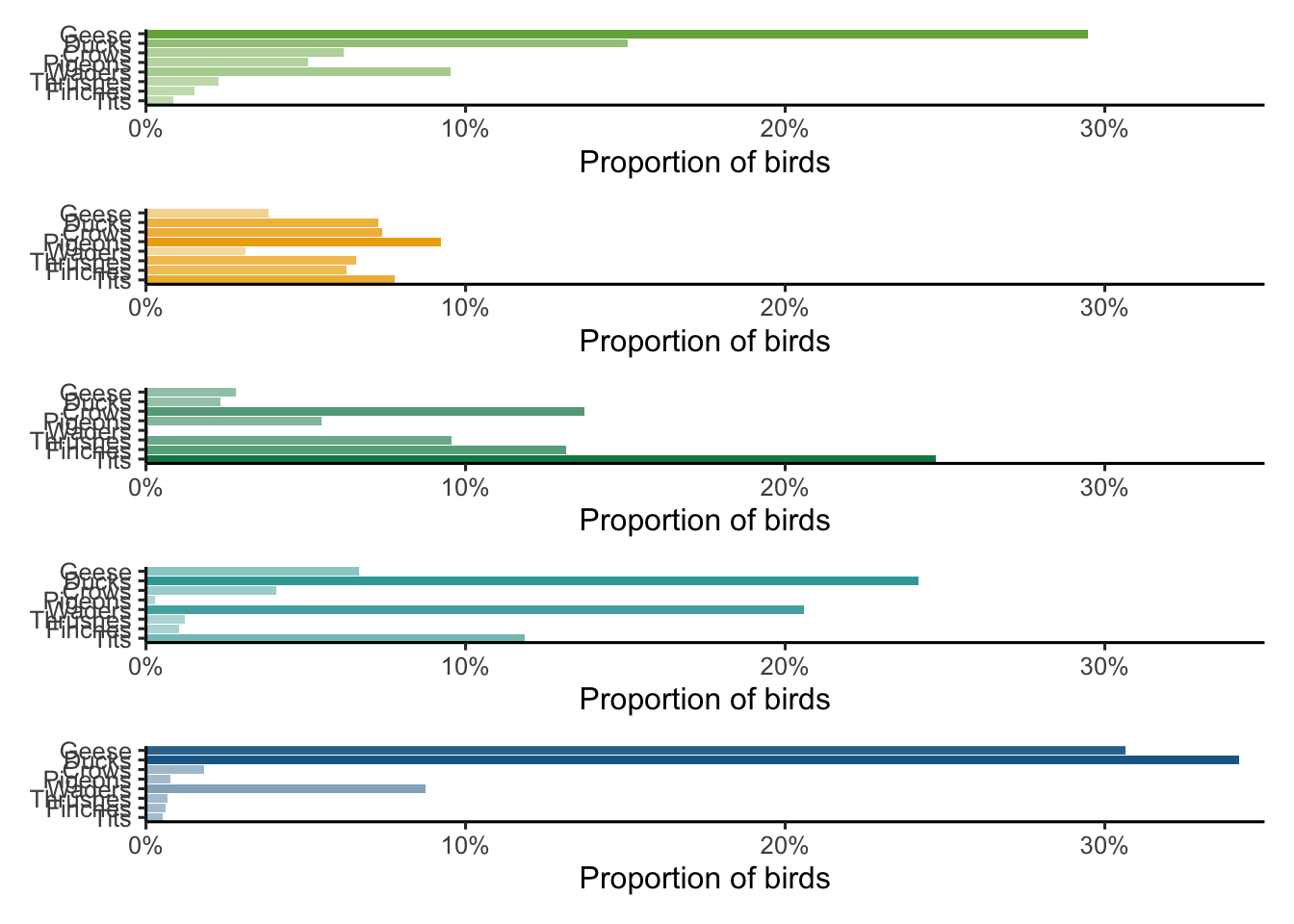
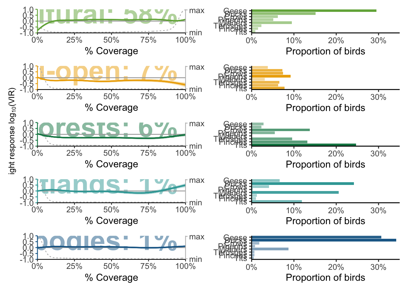
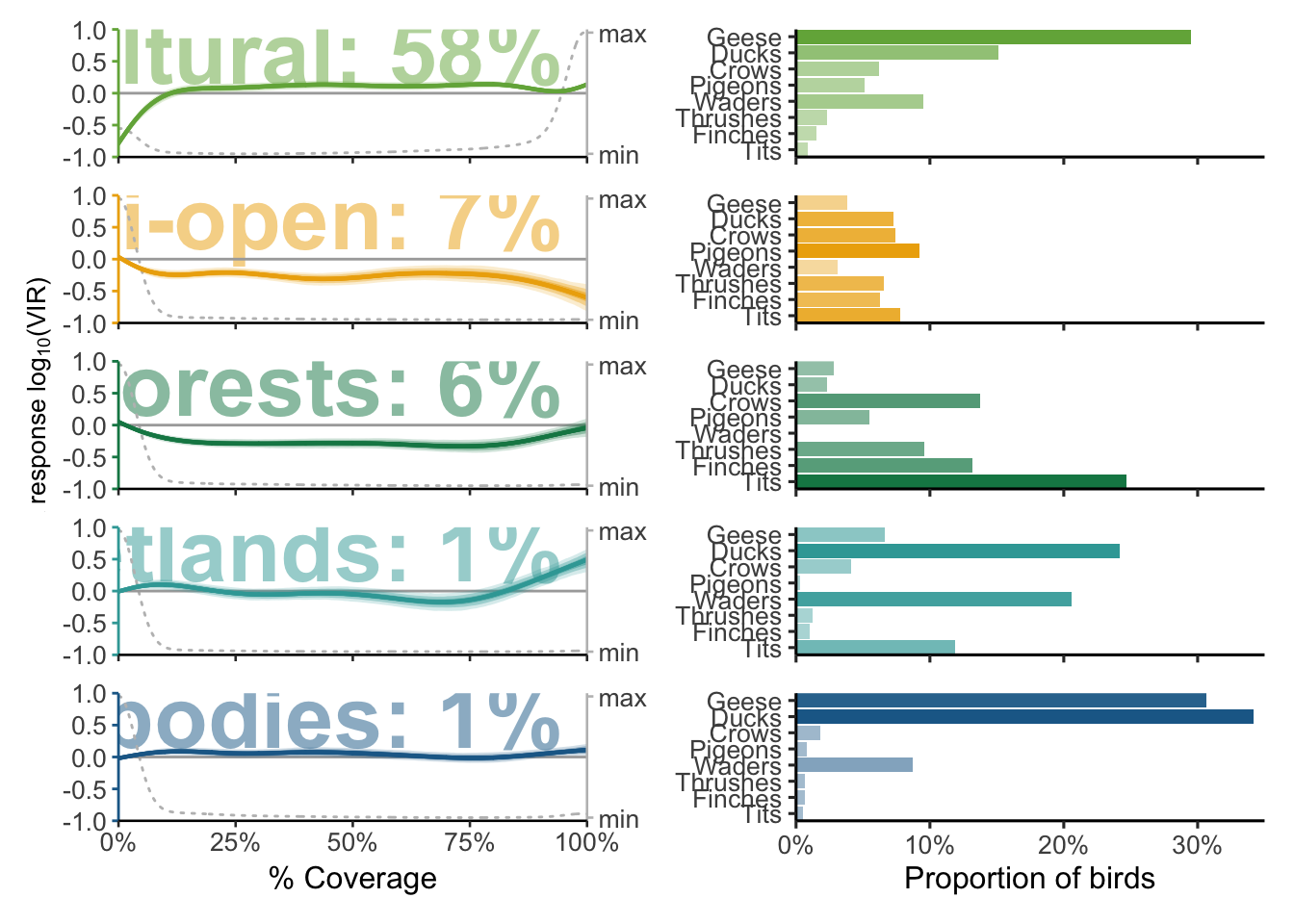
13 Figure 3: Species composition

To illustrate how species composition changes with habitat types, we make a variety of plots:

The top-5 taxonomic families per habitat type.
The proportions of birds that belong to a selection of families that are representative for the entire Dutch landscape.

To quantify the necessary variables we rely mostly on the point-transect counts from Sovon as these cover all species (instead of the waterbird counts).

13.1 Processing environment

library(bioRad)
library(ggplot2)
library(dplyr)
library(tidyr)
library(stringr)
library(ggpointdensity)
library(patchwork)
library(GGally)
library(tibble)
library(ggpubr)
library(forcats)

We load the study PPI and proportions of taxonomic groups in the counts.

ppi <- readRDS("data/processed/composite-ppis/500m/201712312305.RDS")
wb_props <- readRDS("data/processed/sovon/wb_props.RDS")
ptt <- readRDS("data/processed/sovon/ptt.RDS")
ptt_props <- readRDS("data/processed/sovon/ptt_props.RDS")

ppi$data@data %>%
  # left_join(wb_props, by = c("wb_area_nr" = "area_nr")) %>%
  left_join(ptt_props, by = c("ptt_route" = "route")) %>%
  filter(coverage > 0,
       class != 1,
       total_biomass > 0,
       dist_radar < 66000,
       urban < 0.1) %>%
  identity() -> data

We select only those PPI pixels (and their corresponding counts) which are covered for >99% by a single habitat type.

landuse_limit <- 0.99

13.2 Characteristic families

Geese, ducks, pigeons, thrushes, tits, waders, crows and finches represent a substantial part of the Dutch avifauna across a large range of body sizes. We select these to illustrate how the taxonomic proportions change with habitats.

selected_families <- c("Geese", "Ducks", "Pigeons", "Thrushes", "Tits", "Waders", "Crows", "Finches")

data %>%
  dplyr::select(all_of(c(colnames(ptt_props)[3:45], "semiopen", "forests", "wetlands", "waterbodies", "agricultural"))) %>%
  pivot_longer(cols = all_of(colnames(ptt_props)[3:45]), names_to = "family", values_to = "family_prop") %>%
  pivot_longer(cols = all_of(c("agricultural", "semiopen", "forests", "wetlands", "waterbodies")), names_to = "landuse", values_to = "landuse_prop") %>%
  drop_na() %>%
  filter(family %in% selected_families,
         landuse_prop >= landuse_limit) %>%
  group_by(family, landuse) %>%
  summarise(mean_family_prop = mean(family_prop), .groups = "drop_last") %>%
  pivot_wider(names_from = landuse, values_from = mean_family_prop) %>%
  mutate(family_sc = case_when(family == "Geese" ~ "Anatidae",
                               family == "Ducks" ~ "Anatinae",
                               family == "Pigeons" ~ "Columbidae", 
                               family == "Thrushes" ~ "Turdidae",
                               family == "Tits" ~ "Paridae",
                               family == "Waders" ~ "Charadrii",
                               family == "Crows" ~ "Corvidae",
                               family == "Finches" ~ "Fringillidae")) %>%
  identity() -> characteristic_families
characteristic_families

family	agricultural	forests	semiopen	waterbodies	wetlands	family_sc
Crows	0.0619286	0.1373295	0.0740222	0.0182881	0.0407936	Corvidae
Ducks	0.1508770	0.0233594	0.0726795	0.3419478	0.2416624	Anatinae
Finches	0.0152677	0.1314283	0.0628657	0.0062778	0.0102175	Fringillidae
Geese	0.2946680	0.0281144	0.0384954	0.3065711	0.0666727	Anatidae
Pigeons	0.0508753	0.0549949	0.0921633	0.0077864	0.0028696	Columbidae
Thrushes	0.0228345	0.0957379	0.0658859	0.0068034	0.0121501	Turdidae
Tits	0.0084950	0.2470226	0.0778224	0.0051277	0.1186220	Paridae
Waders	0.0953540	0.0006251	0.0310129	0.0873656	0.2058158	Charadrii

13.3 Mean habitat biomass and weight

We calculate the mean biomass for all areas covered for >99% by a single habitat type and calculate mean bird weight for these areas from the point-transect counts.

data %>%
  dplyr::select(all_of(c("total_biomass", "ptt_weighted_mean_weight", "semiopen", "forests", "wetlands", "waterbodies", "agricultural"))) %>%
  pivot_longer(cols = all_of(c("semiopen", "forests", "wetlands", "waterbodies", "agricultural")), names_to = "landuse", values_to = "proportion") %>%
  filter(proportion >= landuse_limit) %>%
  mutate(total_biomass = total_biomass / 1000) %>%
  group_by(landuse) %>%
  summarise(mean_biomass = mean(total_biomass),
            mean_weight = mean(ptt_weighted_mean_weight, na.rm = TRUE),
            .groups = "drop_last") %>%
  arrange(desc(mean_weight)) %>%
  identity() -> habitat_mass
habitat_mass

landuse	mean_biomass	mean_weight
waterbodies	100.098362	1367.6172
agricultural	133.003369	1256.0901
wetlands	213.892151	866.0075
semiopen	31.895918	742.2743
forests	4.002946	246.8706

13.4 Sorting of families by weight

Now we sort families according to weight

ptt %>%
  distinct(species, .keep_all = TRUE) %>%
  group_by(familyvernacular) %>%
  summarise(mean_weight = mean(mean_weight), .groups = "drop_last") %>%
  filter(familyvernacular %in% selected_families) %>%
  arrange(desc(mean_weight)) %>%
  rowid_to_column()-> family_weights

characteristic_families %>%
  left_join(family_weights, by = c("family" = "familyvernacular")) %>%
  arrange(desc(mean_weight)) -> characteristic_families

characteristic_families$rank <- factor(characteristic_families$mean_weight, ordered = TRUE, levels = characteristic_families$mean_weight)

13.5 Prepare plot

And plot a simple barplot figure.

characteristic_families %>%
  pivot_longer(cols = !c("family", "rowid", "mean_weight", "rank", "family_sc"), names_to = "landuse", values_to = "family_prop") -> cf_long

colors <- c("urban" = "#94346E", "agricultural" = "#73AF48", "semiopen" = "#EDAD08", "forests" = "#0F8554", "wetlands" = "#38A6A5", "waterbodies" = "#1D6996",
            "dist_urban" = "#94346E", "total_biomass" = "#CC503E", "dist_radar" = "#666666")
landuse_names <- c("agricultural" = "Agricultural", "semiopen" = "Semi-open", "forests" = "Forests", "wetlands" = "Wetlands", "waterbodies" = "Water bodies")

plot_family_proportions <- function(props, which) {
  landuse_labeller <- function(variable, value) {
    label <- paste0(landuse_names[value], " ", round(habitat_mass[habitat_mass$landuse == which, ]$mean_weight, digits = 0), "g")
    return(label)
  }
  
  proportion_labeller <- function(value) paste0(value * 100, "%")
  
  props %>%
  filter(landuse == which) %>%
  ggplot() +
    geom_col(aes(x = family_prop, y = reorder(family, mean_weight), alpha = family_prop), fill = colors[which]) +
    labs(x = "Proportion of birds", y = "Taxonomic group") +
    coord_cartesian(expand = FALSE, xlim = c(0, ceiling(max(cf_long$family_prop) * 100) / 100)) +
    scale_x_continuous(breaks = c(0, 0.1, 0.2, 0.3), labels = proportion_labeller) +
    scale_alpha_continuous(range = c(0.4, 1)) +
    facet_wrap(vars(landuse), strip.position = "top") +
    theme_classic(base_size = 12) +
    theme(legend.position = "none",
          axis.title.y = element_blank(),
          strip.background = element_blank(),
          strip.text.x = element_blank())
}

landuses <- c("agricultural", "semiopen", "forests", "wetlands", "waterbodies")  # Same order as model outputs

plots <- mapply(function(landuses) { plot_family_proportions(cf_long, landuses) }, landuses = landuses,
            SIMPLIFY = FALSE)

# characteristic_families$title <- "Mean weight (g)"
# ggplot(characteristic_families) +
#   geom_col(aes(x = mean_weight, y = reorder(family, mean_weight))) +
#   labs(x = "Mean weight (g)", y = "Taxonomic group") +
#     coord_cartesian(expand = FALSE) +
#     scale_x_continuous(breaks = c(0, 1000, 2000, 3000)) +
#     facet_wrap(vars(title), strip.position = "top") +
#     theme_classic(base_size = 12) +
#     theme(legend.position = "none",
#           axis.title.y = element_blank(),
#           strip.background = element_blank(),
#           strip.text.x = element_text(hjust = 0, size = 12, family = "Helvetica", face = "bold")) -> plots[[6]]
p <- wrap_plots(plots, ncol = 1)
p

p_models <- readRDS("data/plots/paper/fig_landscapes.RDS")

p_models[[1]] + p_models[[2]] + p_models[[3]] + p_models[[4]] + p_models[[5]] +
  plots[[1]] + plots[[2]] + plots[[3]] + plots[[4]] + plots[[5]] +
  plot_layout(widths = c(1, 1), nrow = 5, byrow = FALSE) & 
  theme(axis.text.x = element_text(size = 10),
        axis.title.x = element_text(size = 12),
        axis.text.y = element_text(size = 10)) -> p_landscape_characterisation

ggsave(filename = "data/plots/paper/fig2_landscape.pdf", plot = p_landscape_characterisation, width = 14, height = 25, dpi = 300, units = "cm")
p_landscape_characterisation

widths <- c(1, 1)
(p_models[[1]] / plots[[1]] * theme(axis.text.x = element_blank(), axis.title.x = element_blank(), axis.text.y = element_text(size = 10)) +
   plot_layout(widths = widths, ncol = 2)) /
  (p_models[[2]] / plots[[2]] * theme(axis.text.x = element_blank(), axis.title.x = element_blank(), axis.text.y = element_text(size = 10)) +
     plot_layout(widths = widths, ncol = 2)) /
  (p_models[[3]] / plots[[3]] * theme(axis.text.x = element_blank(), axis.title.x = element_blank(), axis.text.y = element_text(size = 10)) +
     plot_layout(widths = widths, ncol = 2)) /
  (p_models[[4]] / plots[[4]] * theme(axis.text.x = element_blank(), axis.title.x = element_blank(), axis.text.y = element_text(size = 10)) +
     plot_layout(widths = widths, ncol = 2)) / 
  (p_models[[5]] / plots[[5]] * theme(axis.text.x = element_text(size = 10), axis.title.x = element_text(size = 12), axis.text.y = element_text(size = 10)) +
     plot_layout(widths = widths, ncol = 2)) -> p_landscape_characterisation

p_landscape_characterisation

And we save it as .pdf for editing in Illustrator.

ggsave(filename = "data/plots/paper/fig2_landscape.pdf", plot = p_landscape_characterisation, width = 12, height = 18, dpi = 300, units = "cm")

12 Figure 2: Model output

14 Figure 4: Distance to fireworks