10 Determine baseline disturbance

To compare the disturbance caused by fireworks against the flight activity of normal nights, we select (mostly) rain-free nights from the baseline dataset.

library(ggplot2)
library(dplyr)
library(readr)
library(tidyr)
library(bioRad)

We have previously calculated the classes targets using the depolarization ratio (Kilambi, Fabry, and Meunier 2018) and can now visualise them.

files <- Sys.glob(file.path("data/processed/composite-ppis-baseline/500m", "*"))
lapply(files, function(x) {
  ppi <- readRDS(x)
  plot(ppi, param = "class", zlim = c(0, 2)) + ggtitle(basename(x))
})

## [[1]]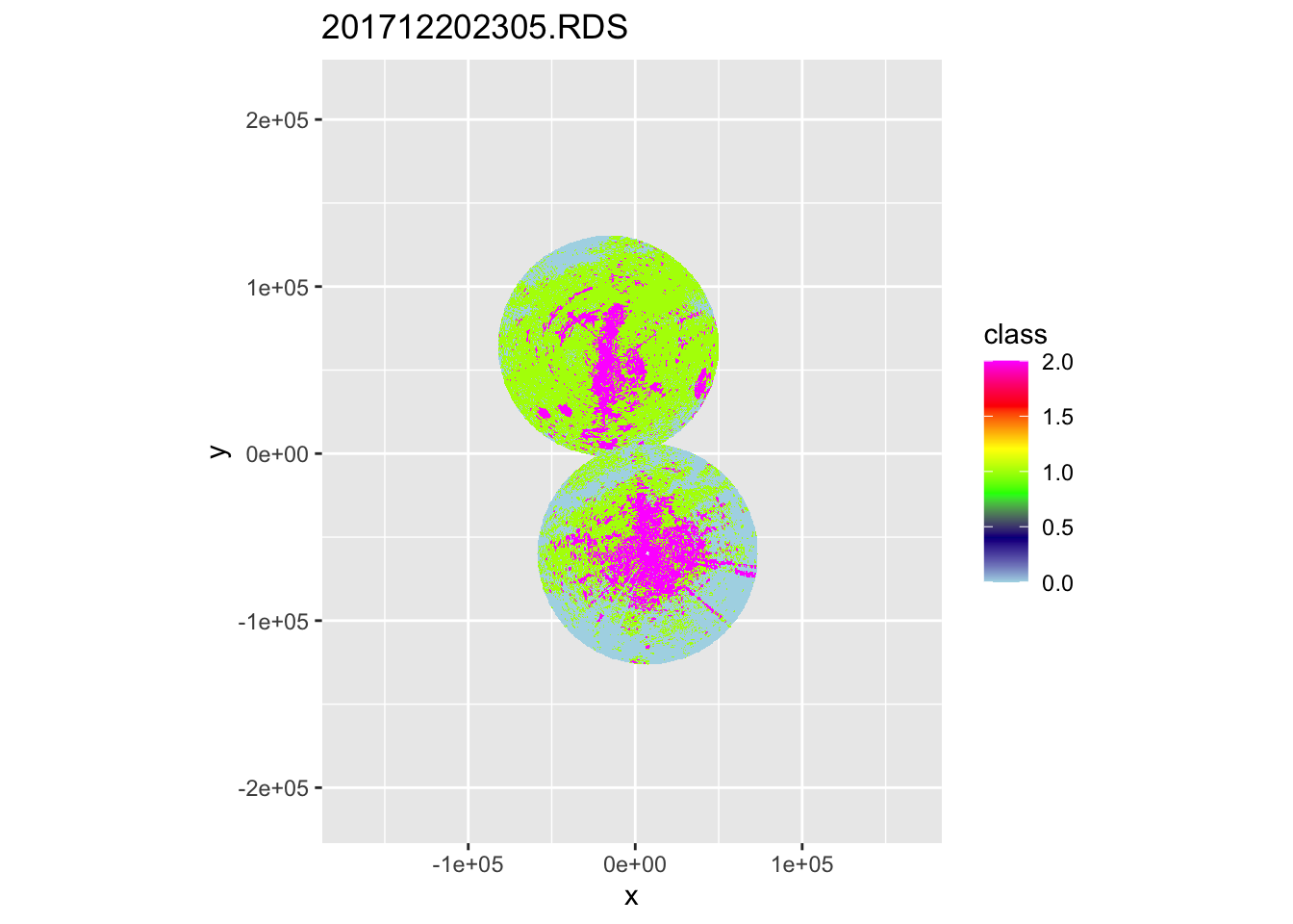

## 
## [[2]]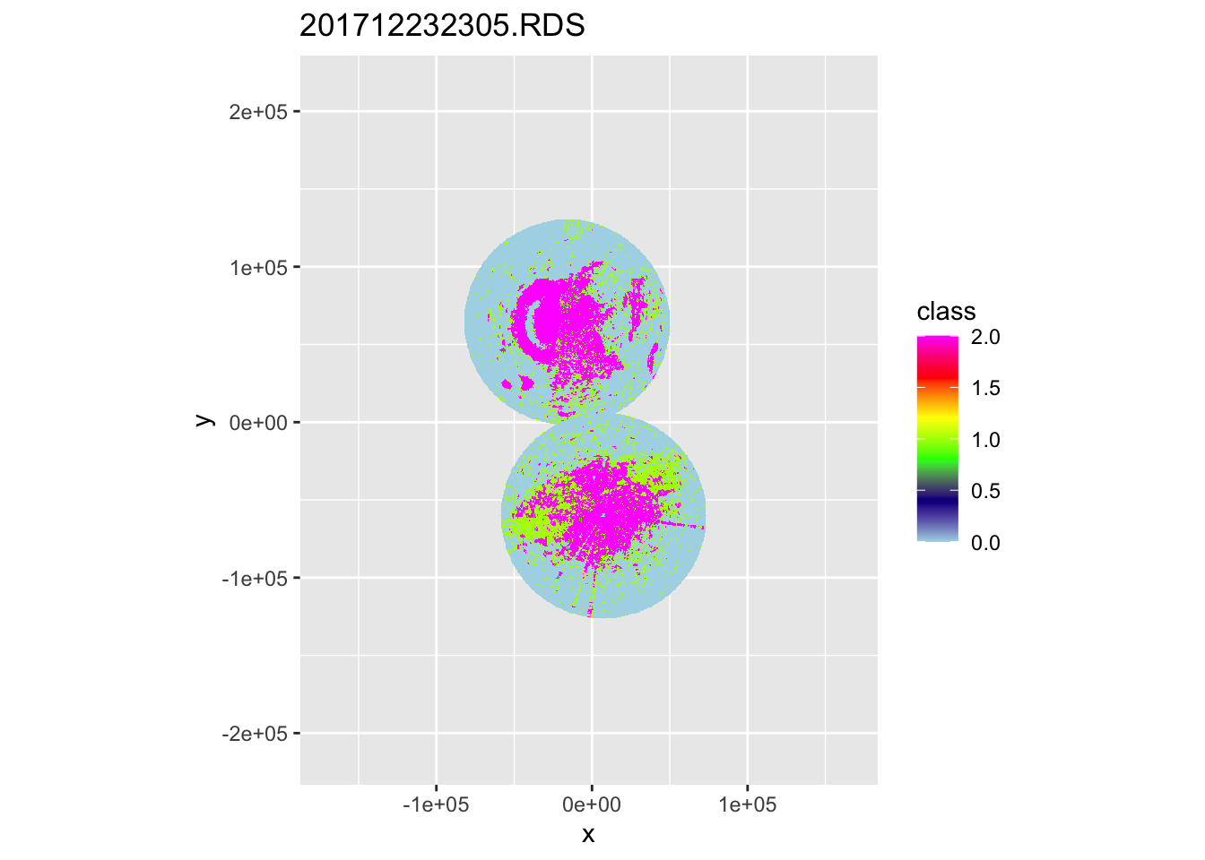

## 
## [[3]]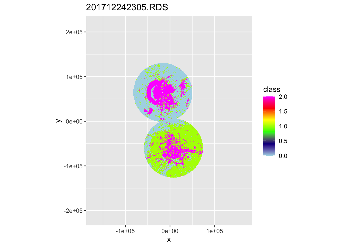

## 
## [[4]]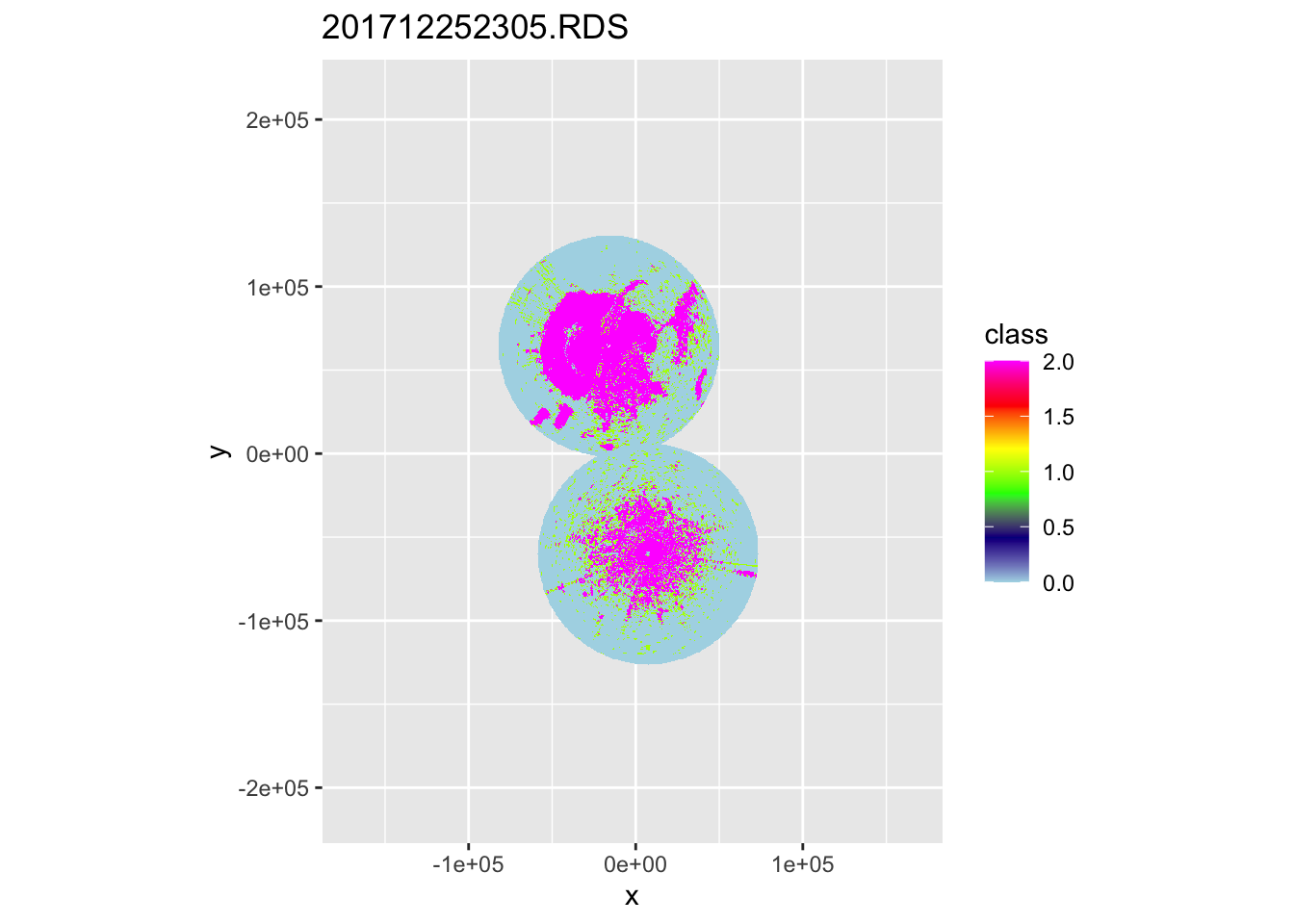

## 
## [[5]]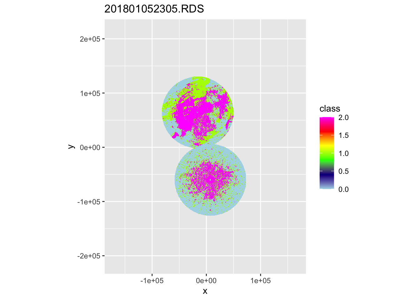

## 
## [[6]]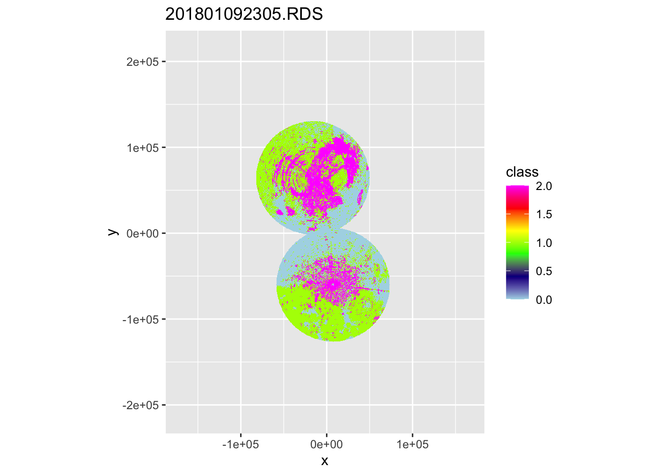

## 
## [[7]]

## 
## [[8]]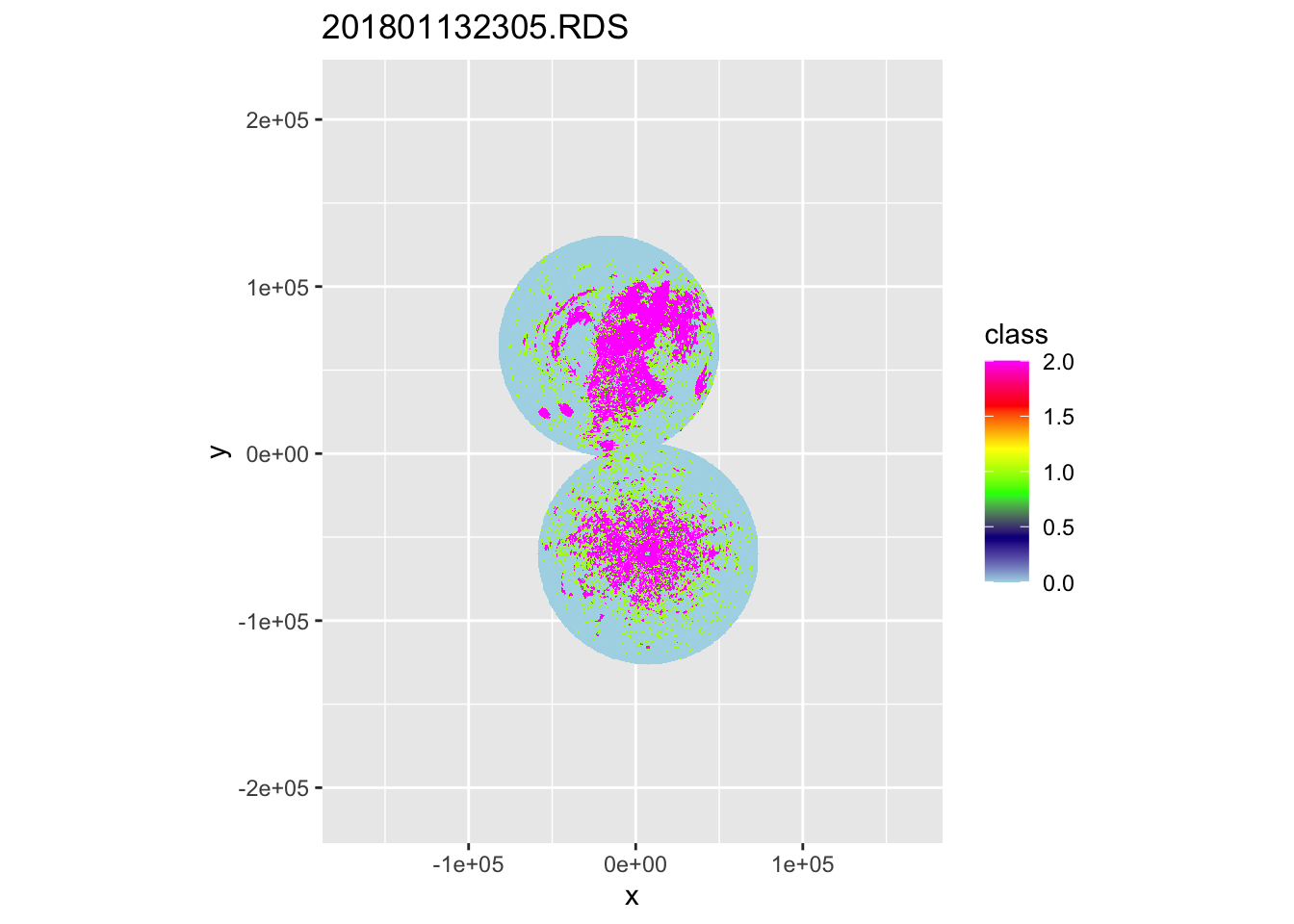

## 
## [[9]]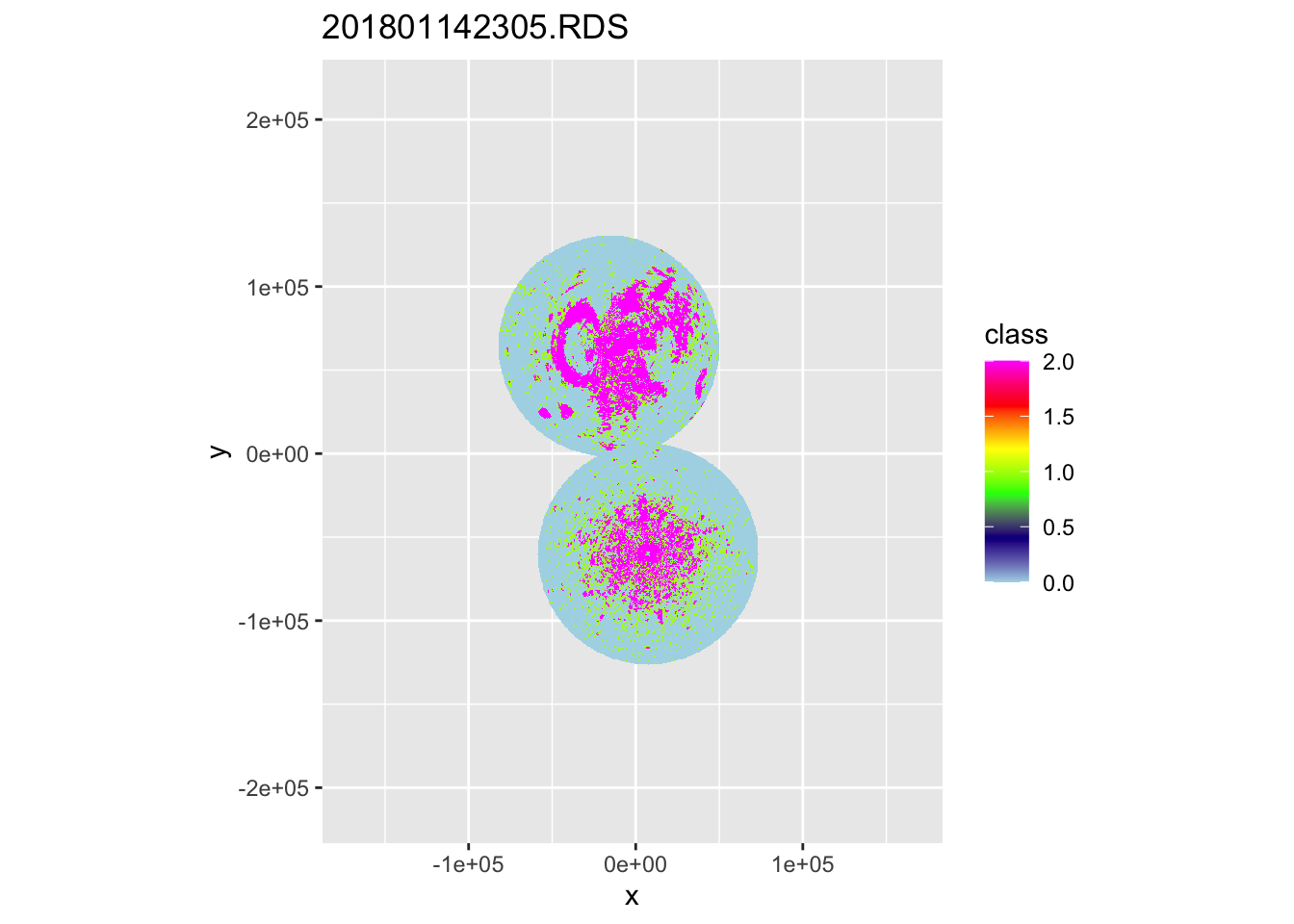

## 
## [[10]]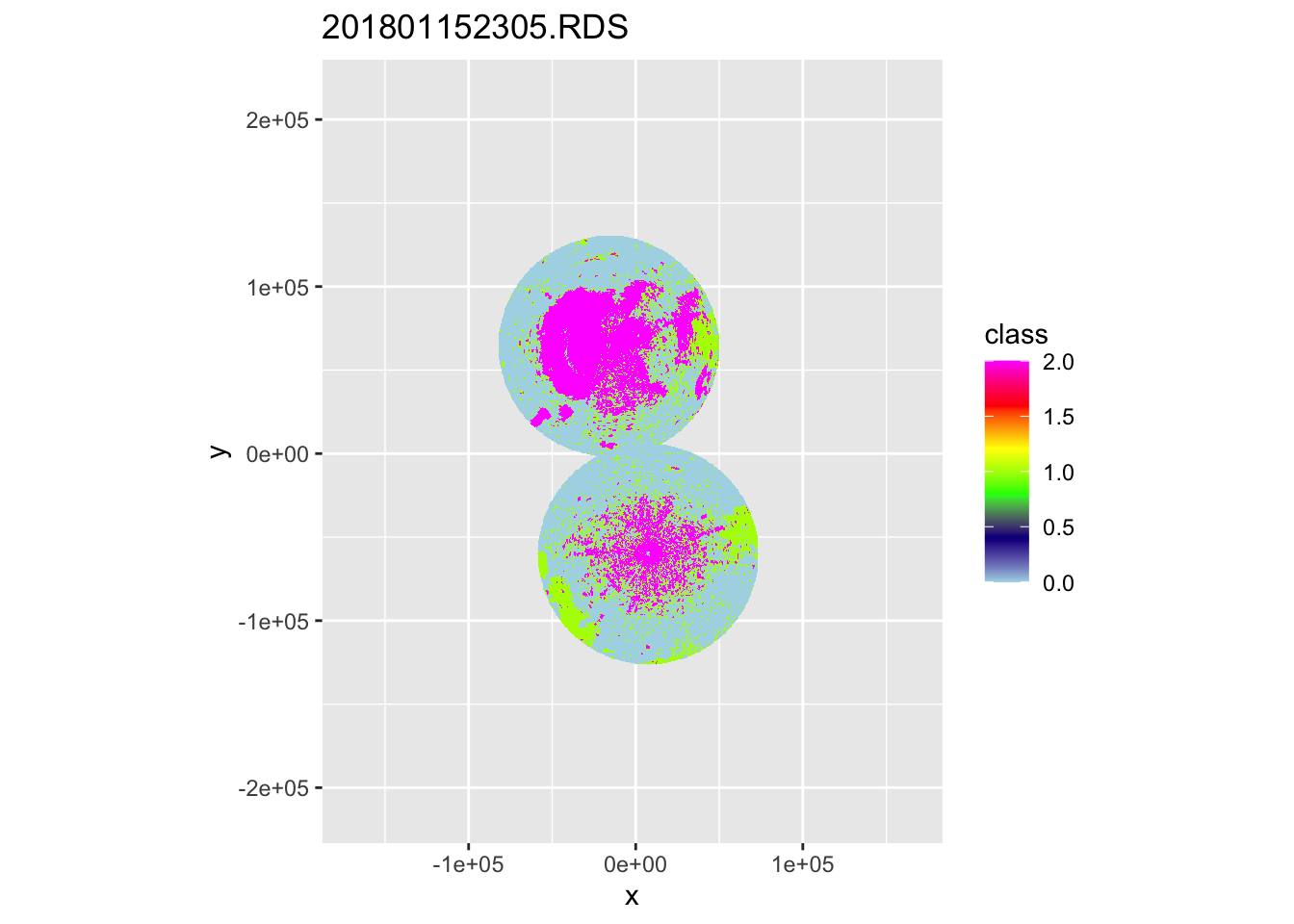

Through visual inspection we’ve determined the following PPIs to be sufficient to serve as a disturbance baseline. They may still contain forms of non-meteorological clutter, but that is not a problem as long as the clutter does not intersect with the count sites.

files_selected <- files[c(2, 4, 6, 7, 8)]

Process the baseline PPIs the same way the disturbed PPIs are processed.

data_disturbance <- readRDS("data/models/data_cleaned.RDS")

data_baseline <- lapply(files_selected, function(x) {
  df <- readRDS(x)[["data"]]@data
  df["dt"] <- basename(tools::file_path_sans_ext(x))
  df
})

clean_data_baseline <- function(data, max_distance, pixels) {
  mdl_variables <- c("VIR", "dist_radar", "total_biomass", "total_crs",
                     "agricultural", "semiopen", "forests", "wetlands", "waterbodies", "urban",
                     "dist_urban", "human_pop", "pixel", "coverage", "class", "x", "y", "dt", "VIDc")
  log10_variables <- c("dist_urban", "human_pop", "total_biomass", "dist_urban")
  
  data %>%
    dplyr::filter(pixel %in% pixels) %>%
    mutate(VIR = replace_na(VIR, 0.1),
           VIR = if_else(VIR == 0, 0.1, VIR),
           VIR = log10(VIR),
           VIDc = (10^VIR) / weighted_mean_crs,
           VIDc = if_else(VIDc > 10000000, 1e-6, VIDc, 1e-6),
           dt = as.factor(dt)) %>%
    dplyr::select(all_of(mdl_variables)) %>%
    filter_all(all_vars(is.finite(.))) %>%
    rename(total_rcs = total_crs) %>%
    identity() -> data_cleaned
  
  data_cleaned
}

baseline_ppis <- lapply(data_baseline, function(x) clean_data_baseline(x, 66000, data_disturbance$pixel))
saveRDS(baseline_ppis, "data/processed/baseline_ppis.RDS")

baseline_response_VIR <- unlist(lapply(baseline_ppis, function(x) mean(x$VIR)))
baseline_response_VIDc <- unlist(lapply(baseline_ppis, function(x) mean(x$VIDc)))
br <- c("VIR" = mean(baseline_response_VIR), "VIDc" = mean(baseline_response_VIDc))
saveRDS(br, file = "data/processed/disturbance_baseline.RDS")
br

##        VIR       VIDc 
## -0.3654903  2.7240716