8 Modelling fireworks disturbance

We have so far:

1. Pre-processed the radar data by removing clutter and applying the range-bias correction (Kranstauber et al. 2020).
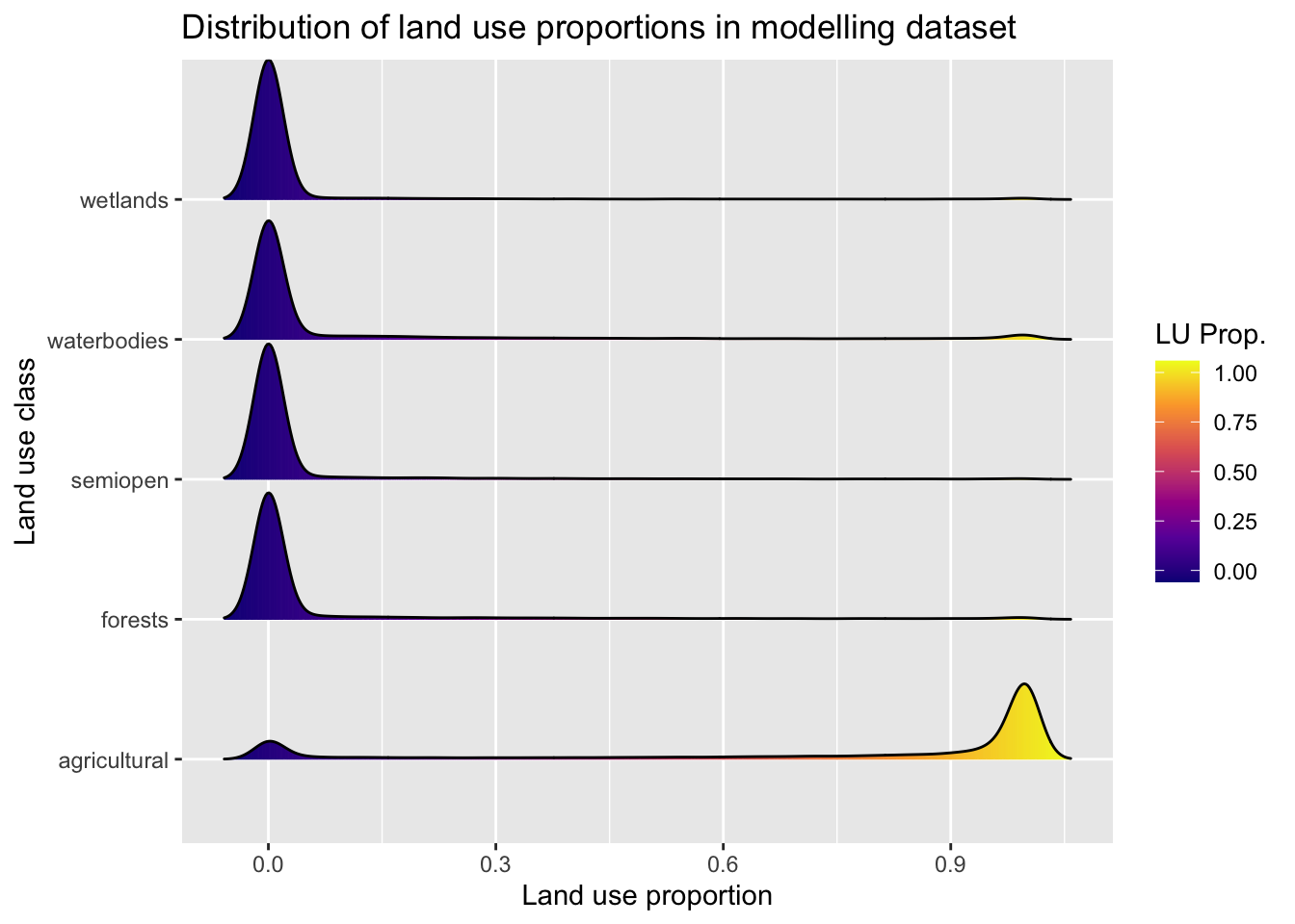
2. Annotated the PPIs with land use proportions and indicators of disturbance, i.e. distance to inhabited urban areas and (human) population density.
3. Annotated the PPIs with the total biomass calculated from the Sovon counts.

With the dataset of annotated PPIs, we can start to explore the relation between fireworks disturbance and the birds measured aloft during NYE 2017-2018.

The following parameters we assume are important predictors for measured bird densities aloft:

1. The total radar cross-section of birds on the ground.
2. The take-off habitat of these birds.
3. The human population in the vicinity of birds.
4. The distance to the nearest inhabited urban area.

8.1 Processing environment

library(ggplot2)
library(dplyr)
library(readr)
library(tidyr)
library(parallel)
library(ggridges)
library(pgirmess)
library(mboost)
library(leaflet)
library(leaflet.opacity)
library(leafem)
library(usdm)
library(mapview)
library(spdep)
library(stringr)

In the previous chapter, we have created some datasets encompassing all the data contained within the individual PPIs at different resolutions. We will determine the optimal resolution and then continue using this dataset for further modelling.

selected_scan <- load("data/processed/pvol_selection.RData")
scan_dt <- str_extract(basename(pvol_dhl_path), "[0-9]{12}")
resolutions <- file.path("data/processed/composite-ppis", c("500m", "1000m", "2000m"), paste0(scan_dt, ".RDS"))
data <- lapply(resolutions, function(x) readRDS(x)[["data"]]@data)
names(data) <- c("500m", "1000m", "2000m")

8.2 Preparing a dataset for modelling

As we’re mostly interested in the moment of en masse take-off of birds, and we want to limit the effects of dispersal, we will limit our analysis to the first 5 minutes after 00:05 on January 1st, 2018 (or 23:05 on December 31st, 2017 in UTC), as both radar sites (Den Helder and Herwijnen) show a low VIR prior to and a rapid increase in VIR for that period (see Identifying moment of take-off). Making sure birds are thus still sufficiently ‘linked’ to the take-off sites requires that we limit our analysis to only this one scan.

Furthermore, we want to make sure that:

1. the area is ‘covered’ by at least 1 radar,
2. we have an estimate of total_rcs (and thus total_biomass) for these sites,
3. the proportion of urban area (urban) in the PPI pixel is less than .1,
4. VIR is > 0 (otherwise log-conversion will return -Inf), so we replace 0-values with 1e-3,
5. the radar beam does not overshoot birds too much based on the vp.

clean_data <- function(data, max_distance) {
  mdl_variables <- c("VIR", "dist_radar", "total_biomass", "total_crs",
                     "agricultural", "semiopen", "forests", "wetlands", "waterbodies", "urban",
                     "dist_urban", "human_pop", "disturb_pot", "pixel", "coverage", "class", "x", "y")
  log10_variables <- c("dist_urban", "human_pop", "total_biomass", "dist_urban", "disturb_pot")
  
  data %>%
    dplyr::filter(coverage > 0,
                  class != 1,
                  total_biomass > 0,
                  dist_radar < max_distance,
                  urban < 0.1) %>%
    mutate(VIR = replace_na(VIR, 0.1),
           VIR = if_else(VIR == 0, 0.1, VIR),
           VIR = log10(VIR),
           disturb_pot = human_pop / dist_urban,
           total_biomass = total_biomass / 1000) %>%
    dplyr::select(all_of(mdl_variables)) %>%
    filter_all(all_vars(is.finite(.))) %>%
    rename(total_rcs = total_crs) %>%
    identity() -> data_cleaned
  
  data_cleaned
}

data_cleaned <- lapply(data, function(x) clean_data(x, 66000))
rm(data)

8.3 Determine model resolution based on performance in simple total_crs model

As we want to account for the influence of total_rcs on the measured response by the radars, we will test the performance of a simple model using just dist_radar to correct for range-biased measurement error and total_rcs for the resolutions we have generated composte PPIs for so far (500m, 1000m and 2000m).

Let’s start with a calculation of the RMSE.

resolution_models <- lapply(data_cleaned, function(x) mboost(VIR ~ bbs(dist_radar) + bbs(total_rcs), 
                                                             data = x, control = boost_control(mstop = 10000, trace = TRUE)))
saveRDS(resolution_models, file = "data/models/resolution_models.RDS")

resolution_models <- readRDS("data/models/resolution_models.RDS")
RMSE <- function(error) { sqrt(mean(error^2)) }
sapply(resolution_models, function(x) RMSE(residuals(x)))

##     500m    1000m    2000m 
## 1.236034 1.239162 1.248618

We can also use percentage of deviance explained

deviance_explained <- function(observed, predicted) {
  p <- predicted
  o <- observed
  i <- rep(mean(observed), length(observed))  # Intercept
  total.deviance <- sum((o - i) * (o - i)) / length(observed)  # Deviance from an intercept-only model
  resid.deviance <- sum((o - p) * (o - p)) / length(observed)  # Deviance from the fitted model
  (total.deviance - resid.deviance) / total.deviance
}

mapply(function(data, model) { deviance_explained(data$VIR, predict(model))}, data = data_cleaned, model = resolution_models)

##      500m     1000m     2000m 
## 0.2233546 0.2247612 0.2255258

Turns out most models perform quite similarly. However, to make the link between birds and the habitat they take off from as strong as possible, it makes sense to continue just with the 500m model.

data_cleaned <- data_cleaned$`500m`
saveRDS(data_cleaned, file = "data/models/data_cleaned.RDS")
rm(resolution_models)

8.4 Check for correlations among predictors

We have to see if variables are strongly correlated and thus unfit for being included in the same model, so we calculate Spearman correlation coefficients for all numerical predictors. As this is ecological data, some degree of correlation is of course inevitable for most variables.

mdl_variables <- c("VIR", "dist_radar", "datetime", "total_biomass", "total_rcs", "agricultural", "semiopen", "forests", "wetlands", "waterbodies",
                   "urban", "dist_urban", "human_pop", "disturb_pot", "pixel", "coverage", "class")
predictors <- mdl_variables[!mdl_variables %in% c("VIR", "datetime", "pixel", "x", "y", "coverage", "class")]
corr_radar <- ggstatsplot::ggcorrmat(data_cleaned, output = "plot", type = "spearman", cor.vars = all_of(predictors), colors = c("#2166AC", "#F7F7F7", "#B2182B"))
corr_radar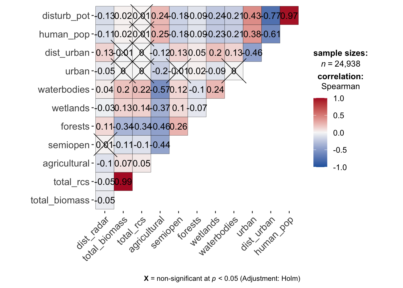

So obviously there is correlation between the disturbance proxies and between agricultural and other land use proportions. For the disturbance proxies it would make sense to determine which is most performant (including all does not make sense), but we can continue using the agricultural predictor as boosted models do not suffer from multicollinearity problems like traditional (e.g.) GAMs.

8.5 Correlated land use proportions

While we’re at it, let’s see what the distributions of values are for the different land use proportions.

data_cleaned %>%
  dplyr::select(agricultural, semiopen, forests, wetlands, waterbodies) %>%
  pivot_longer(cols = everything(), names_to = "landuse", values_to = "value") %>%
  ggplot(aes(x = value, y = landuse, fill = stat(x))) +
  geom_density_ridges_gradient(scale = 1, rel_min_height = 0.0) +
  scale_fill_viridis_c(name = "LU Prop.", option = "C") +
  labs(title = "Distribution of land use proportions in modelling dataset") +
  xlab("Land use proportion") +
  ylab("Land use class")

As can be expected in The Netherlands, the dominant land use class is clearly agricultural with the most prominent peak at full PPI pixel coverage (values close to 1) and all other land use classes peaking very strongly at low proportions. This essentially means that when one of the other land use classes increases in proportion, this will almost always come at the cost of the proportion of agricultural and vice versa.

8.6 Determine the most suitable proxy for disturbance

Now we will compare the disturbance proxies in a similar fashion to how we compared the performance of the model using different PPI resolutions, by calculating deviance explained and RMSE.

fm_dist_urban <- VIR ~ bbs(dist_radar) + bbs(total_rcs) + bbs(semiopen) + bbs(forests) + bbs(wetlands) + bbs(waterbodies) +
  bbs(agricultural) + bbs(dist_urban)
fm_human_pop <- VIR ~ bbs(dist_radar) + bbs(total_rcs) + bbs(semiopen) + bbs(forests) + bbs(wetlands) + bbs(waterbodies) + 
  bbs(agricultural) + bbs(human_pop)
fm_disturb_pot <- VIR ~ bbs(dist_radar) + bbs(total_rcs) + bbs(semiopen) + bbs(forests) + bbs(wetlands) + bbs(waterbodies) + 
  bbs(agricultural) + bbs(disturb_pot)
formulas <- list(fm_dist_urban, fm_human_pop, fm_disturb_pot)

disturbance_models <- lapply(formulas, function(formula) mboost(formula, data = data_cleaned, control = boost_control(mstop = 10000, trace = TRUE)))
names(disturbance_models) <- c("dist_urban", "human_pop", "disturb_pot")
saveRDS(disturbance_models, file = "data/models/disturbance_models.RDS")

disturbance_models <- readRDS("data/models/disturbance_models.RDS")
RMSE <- function(error) { sqrt(mean(error^2)) }
rmse <- sapply(disturbance_models, function(x) RMSE(residuals(x)))
d2 <- mapply(function(model) { deviance_explained(data_cleaned$VIR, predict(model))}, model = disturbance_models)
perf_original <- as.data.frame(list("RMSE" = as.matrix(rmse), "Dev.Exp" = as.matrix(d2)))
perf_original

	RMSE	Dev.Exp
dist_urban	1.136365	0.3435550
human_pop	1.142345	0.3366284
disturb_pot	1.144977	0.3335684

It is clear dist_urban performs the best, though just by a slight margin. As it is probably the most interpretable proxy from a policy perspective, we can thus continue using it without any regrets.

model <- disturbance_models$dist_urban
saveRDS(model, file = "data/models/model.RDS")
rm(disturbance_models)

8.7 Determine the optimal number of boosting steps

The main hyperparameter to be tuned for the boosted GAMs using mboost is the number of boosting iterations/steps. By stopping boosting before model performance (measured using cross-validation) worsens, we can avoid overfitting. We limit this test of model performance for a maximum of 50,000 boosts.

model_boosts <- mboost(fm_dist_urban, data = data_cleaned, control = boost_control(mstop = 1000, trace = FALSE))
saveRDS(model_boosts, file = "data/models/model_boosts.RDS")

grid <- c(1.68^(1:20), 50000)  # Generate a non-linear grid of mstop values to avoid slow convergence

cv10f <- mboost::cv(model.weights(model_boosts), type = "kfold")
saveRDS(cv10f, file = "data/models/boost_cv10f.RDS")

cvm <- cvrisk(model_boosts, folds = cv10f, grid = grid, papply = lapply)
saveRDS(cvm, file = "data/models/cvm_boosts.RDS")

cvm <- readRDS("data/models/cvm_boosts.RDS")
class(cvm) <- NULL
as.data.frame(cvm) %>%
  tibble::rownames_to_column(var = "fold") %>%
  pivot_longer(-c(fold), names_to = "boosts", values_to = "risk") %>%
  mutate(boosts = as.numeric(boosts),
         fold = as.factor(fold)) %>%
  identity() %>%
  ggplot(aes(x = boosts, y = risk, group = fold, color = fold)) +
    geom_line() +
    labs(title = paste0(attr(cvm, "type")), x = "boosts (mstop)", y = attr(cvm, "risk")) +
  scale_x_continuous(trans = "log10")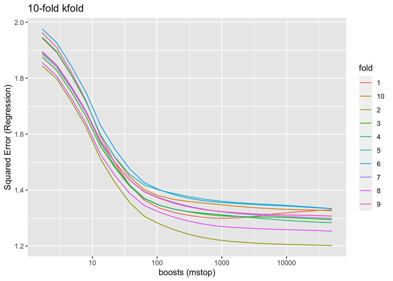

We can see that model performance improves very little beyond a few thousand boosting iterations. As we have to quantify model uncertainty using bootstrapping techniques, it makes little computational sense to push much beyond 10000 boosts, as that would just make the bootstrapping procedure last much longer.

8.8 Variable importance

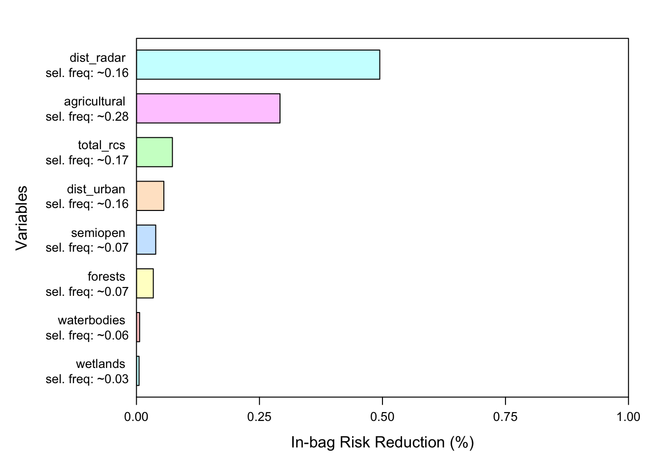
We can quantify the importance of variables within our model using the varimp function which returns variable importance, a measure of the total improvement to model deviance a variable is responsible for.

plot(varimp(model))

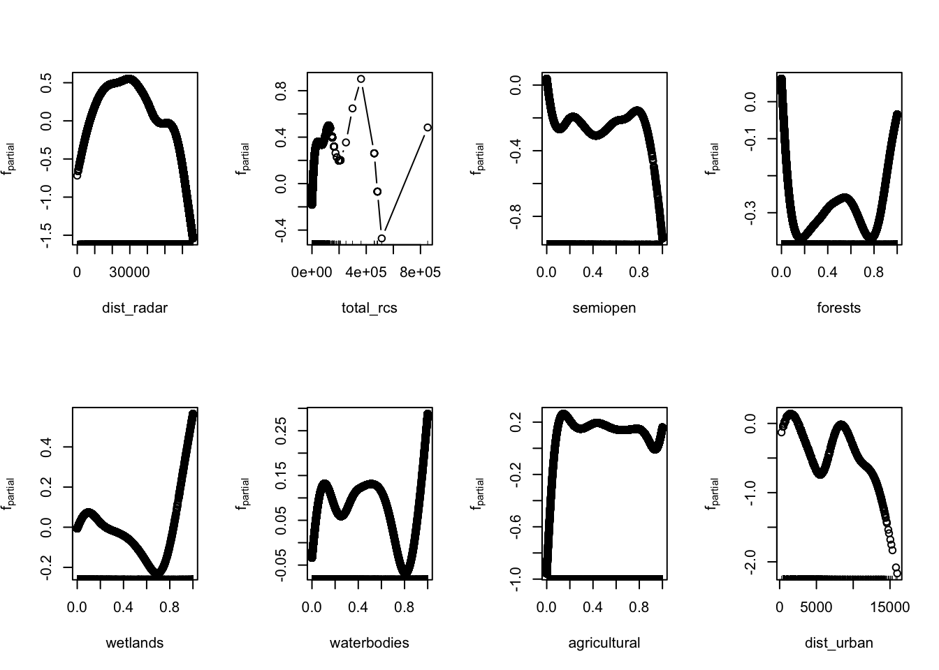
8.9 Model marginal effects

Let’s quickly visualise marginal effects of this model, showing how individual variables influence model outcome with all other variables held constant.

par(mfrow = c(2, 4))
plot(model)

8.10 Spatial autocorrelation

Model residuals should not show strong autocorrelation as then the independency of errors assumption is violated (see for example this). Additionally, a model with strong autocorrelation in the residuals suggests that it lacks a spatial component within the predictors. As it is computationally too difficult to calculate the spatial autocorrelation for the entire dataset at once, we subsample 20% of datapoints for these calculations. Results may thus vary to some degree.

df <- data_cleaned
df$residual <- resid(model)

df %>%
  filter(dist_radar < 66000) %>%
  slice_sample(prop = 0.20) -> df_sample

correlogram <- correlog(df_sample[, c("x", "y")], df_sample[, "residual"], method = "Moran", nbclass = NULL)
saveRDS(correlogram , file = "data/models/correlogram.RDS")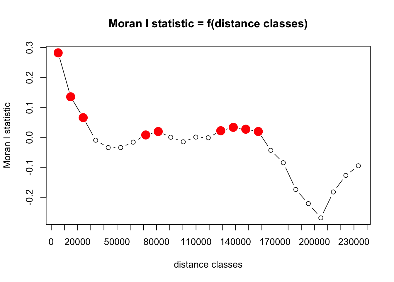

correlogram <- readRDS("data/models/correlogram.RDS")
plot(correlogram)

This shows there’s some spatial autocorrelation in residuals remaining. We use a plot of residuals to assess where this occurs and if this indicates our model is missing some important spatial effect, or if there is another explanation.

Unfortunately, due to the way leaflet stores maps it produces, we cannot plot them here using K-M knitting to generate this document. Run these chunks interactively and they should work fine. So, here we’ll have to resort to a static representation of the model residuals.

df <- data_cleaned
df$residual <- resid(model)
df$preds <- predict.mboost(model, newdata = data_cleaned)
ppi <- readRDS("data/processed/composite-ppis/500m/201712312305.RDS")
 
ppi$data@data %>%
  left_join(dplyr::select(df, pixel, preds, residual), by = "pixel") -> ppi$data@data
ppi$data@data$VIR_log <- log10(ppi$data@data$VIR)
ppi$data@data$total_biomass_log <- log10(ppi$data@data$total_biomass / 1000)

pal_resid <- colorspace::diverging_hcl(50, "Blue-Red 3", power = 2)
z_lims_resid <- c(-3, 3)
palette_resid <- colorNumeric(pal_resid, na.color = "#00000005", domain = z_lims_resid)
raster_resid <- as(ppi$data["residual"], "RasterLayer")
raster_resid[raster_resid <= z_lims_resid[1]] <- z_lims_resid[1]
raster_resid[raster_resid >= z_lims_resid[2]] <- z_lims_resid[2]

leaflet() %>%
  addTiles(group = "OSM (default)") %>%
  addRasterImage(raster_resid, colors = palette_resid, layerId = "resid", group = "resid") %>%
  addImageQuery(raster_resid, layerId = "resid") %>%
  addLegend(pal = palette_resid, values = z_lims_resid) %>%
  addOpacitySlider(layerId = "resid") %>%
  identity()

as.data.frame(raster_resid, xy = TRUE) %>%
  drop_na() %>%
  ggplot() +
  geom_raster(aes(x = x, y = y, fill = residual)) +
  scale_fill_distiller(type = "div", palette = "RdBu") +
  theme_dark()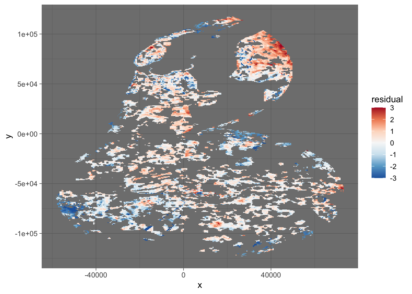

8.10.1 Correct for residual spatial autocorrelation

The correlogram and spatial plots of residuals show clearly that residuals are spatially autocorrelated. We will correct for this effect using Crase et al. (2012), by calculating an autocovariate (distance weighted mean) of the residuals using a 1500m neighborhood radius. If we look at the correlogram above, we can see that spatial autocorrelation is still visible at distances of 30-50km, but calculating an autocovariate for such neighborhoods would be too computationally intensive. Some points won’t have neighborhoods at all, but that is fine.

nbs <- 1500  # Kilometers if longlat = TRUE
acov <- autocov_dist(resid(model), as.matrix(cbind(data_cleaned$x, data_cleaned$y)), nbs = nbs, zero.policy = TRUE)

## Warning in autocov_dist(resid(model), as.matrix(cbind(data_cleaned$x,
## data_cleaned$y)), : With value 1500 some points have no neighbours

## Warning in nb2listw(nb, glist = gl, style = style, zero.policy = zero.policy):
## zero sum general weights

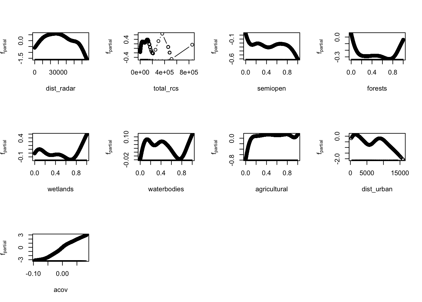
data_cleaned$acov <- acov

Having calculated the autocovariate and included it in our dataset, we can retrain a model, this time with the inclusion of the autocov parameter.

formula <- VIR ~ bbs(dist_radar) + bbs(total_rcs) + bbs(semiopen) + bbs(forests) + bbs(wetlands) + bbs(waterbodies) +
  bbs(agricultural) + bbs(dist_urban) + bbs(acov)
model_rac <- mboost(formula, data = data_cleaned, control = boost_control(mstop = 10000, trace = TRUE))
saveRDS(model_rac, file = "data/models/model_rac.RDS")

Let’s plot model variable importance and modelled effects again for this newly trained model.

model_rac <- readRDS("data/models/model_rac.RDS")
plot(varimp(model_rac))

par(mfrow = c(3, 4))
plot(model_rac)

And recalculate Moran’s I for the new model residuals.

df <- data_cleaned
df$residual <- resid(model_rac)

df %>%
  filter(dist_radar < 66000) %>%
  slice_sample(prop = 0.2) -> df_sample

correlogram <- correlog(df_sample[, c("x", "y")], df_sample[, "residual"], method = "Moran", nbclass = NULL)
saveRDS(correlogram , file = "data/models/correlogram_rac.RDS")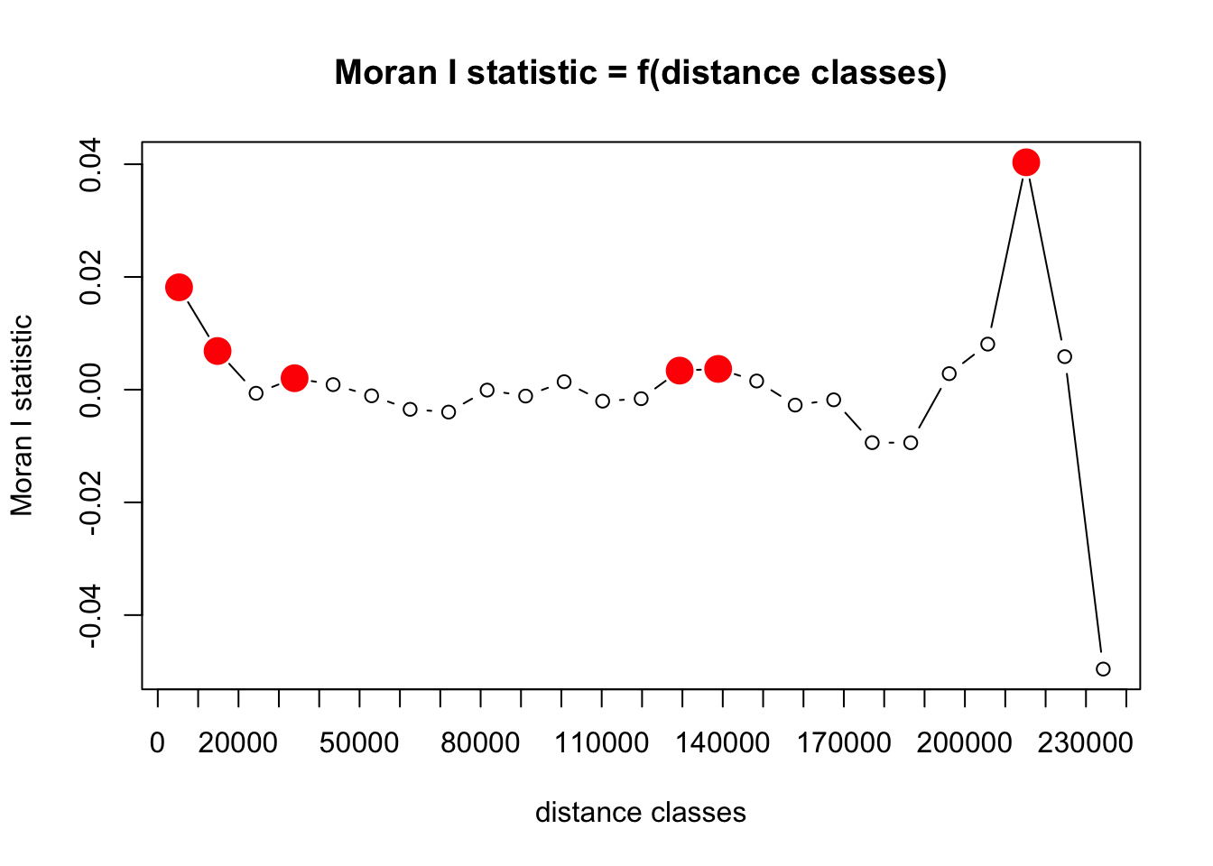

correlogram <- readRDS("data/models/correlogram_rac.RDS")
plot(correlogram)

That looks much better! Residual spatial autocorrelation is still present and significant (red circles in plot above), but has now decreased from ~0.3 to ~0.02. So it is now pretty much negligible.

For completeness, let’s make the residuals spatially explicit again

df <- data_cleaned
df$residual <- resid(model_rac)
df$preds <- predict.mboost(model_rac, newdata = data_cleaned)
ppi <- readRDS("data/processed/composite-ppis/500m/201712312305.RDS")
 
ppi$data@data %>%
  left_join(dplyr::select(df, pixel, preds, residual), by = "pixel") -> ppi$data@data
ppi$data@data$VIR_log <- log10(ppi$data@data$VIR)
ppi$data@data$total_biomass_log <- log10(ppi$data@data$total_biomass / 1000)

pal_resid <- colorspace::diverging_hcl(50, "Blue-Red 3", power = 2)
z_lims_resid <- c(-3, 3)
palette_resid <- colorNumeric(pal_resid, na.color = "#00000005", domain = z_lims_resid)
raster_resid <- as(ppi$data["residual"], "RasterLayer")
raster_resid[raster_resid <= z_lims_resid[1]] <- z_lims_resid[1]
raster_resid[raster_resid >= z_lims_resid[2]] <- z_lims_resid[2]

leaflet() %>%
  addTiles(group = "OSM (default)") %>%
  addRasterImage(raster_resid, colors = palette_resid, layerId = "resid", group = "resid") %>%
  addImageQuery(raster_resid, layerId = "resid") %>%
  addLegend(pal = palette_resid, values = z_lims_resid) %>%
  addOpacitySlider(layerId = "resid") %>%
  identity()

as.data.frame(raster_resid, xy = TRUE) %>%
  drop_na() %>%
  ggplot() +
  geom_raster(aes(x = x, y = y, fill = residual)) +
  scale_fill_distiller(type = "div", palette = "RdBu") +
  theme_dark()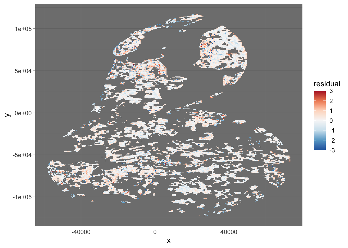

And finally we can recalculate the model performance and compare it with the original model.

RMSE <- function(error) { sqrt(mean(error^2)) }
rmse <- RMSE(residuals(model_rac))
de <- deviance_explained(data_cleaned$VIR, predict(model_rac))
perf_rac <- as.data.frame(list("RMSE" = as.matrix(rmse), "Dev.Exp" = as.matrix(de)))

perf <- bind_rows(perf_original["dist_urban", ], perf_rac)
rownames(perf) <- c("dist_urban_original", "dist_urban_rac")
perf

	RMSE	Dev.Exp
dist_urban_original	1.136365	0.3435550
dist_urban_rac	0.707957	0.7450364