3 Species assemblage trends
In this study we follow the methodology of Beresford et al. 3 and calculate an assemblage trend across our entire study area. If we assume environmental factors in wintering areas (in this case Africa) play some role towards influencing species trends, areas where assemblage trends (the product of individual species trends) are higher are more likely to provide beneficial environmental factors and vice versa.
3.1 Calculate assemblage trends
We calculate long- and short-term assemblage trends based on the PECBMS long-term and short-term trends. We use the raster of NDVI predictability as a template to project these values onto. Additionally, we will calculate the number of species that occur within these assemblages.
trendspecies <- readRDS("data/processed/trendspecies.RDS")

trend_long_raster <- list()
trend_short_raster <- list()

template_raster <- raster::raster("data/raw/gee/ndvi_1.tif")

# Rasterize distribution maps of individual species and assign trend to pixel values
for (i in 1:nrow(trendspecies)) {
  trend_long_raster[[i]] <- fasterize(trendspecies[i, ], raster = template_raster, field = "trend_long")
  trend_short_raster[[i]] <- fasterize(trendspecies[i, ], raster = template_raster, field = "trend_short")
}

# Turn list of rasters into raster bricks for calculations
trend_long_raster <- suppressWarnings(brick(trend_long_raster))
trend_short_raster <- suppressWarnings(brick(trend_short_raster))
names(trend_long_raster) <- trendspecies[, "species"]$species
names(trend_short_raster) <- trendspecies[, "species"]$species

# Calculate assemblage trend
trend_long_assemblage <- calc(trend_long_raster, mean, na.rm = TRUE)
trend_short_assemblage <- calc(trend_short_raster, mean, na.rm = TRUE)

# Reclassify trends to NA or 1
trend_long_counts <- suppressWarnings(reclassify(trend_long_raster, c(-Inf, Inf, 1)))
trend_short_counts <- suppressWarnings(reclassify(trend_short_raster, c(-Inf, Inf, 1)))

# Calculate number of species that make up an assemblage
trend_long_counts <- calc(trend_long_counts, sum, na.rm = TRUE)
trend_short_counts <- calc(trend_short_counts, sum, na.rm = TRUE)

# Write rasters to files
writeRaster(trend_long_assemblage, file = "data/processed/trend_long_assemblage.tif", overwrite = TRUE)
writeRaster(trend_short_assemblage, file = "data/processed/trend_short_assemblage.tif", overwrite = TRUE)
writeRaster(trend_long_counts, file = "data/processed/trend_long_counts.tif", overwrite = TRUE)
writeRaster(trend_short_counts, file = "data/processed/trend_short_counts.tif", overwrite = TRUE)
3.2 Plot assemblage trends
Let’s make a quick plot of the assemblage trends side by side
par(mfrow = c(1, 2))
plot(trend_long_assemblage, main = "Long-term assemblage trend")
plot(trend_short_assemblage, main = "Short-term assemblage trend")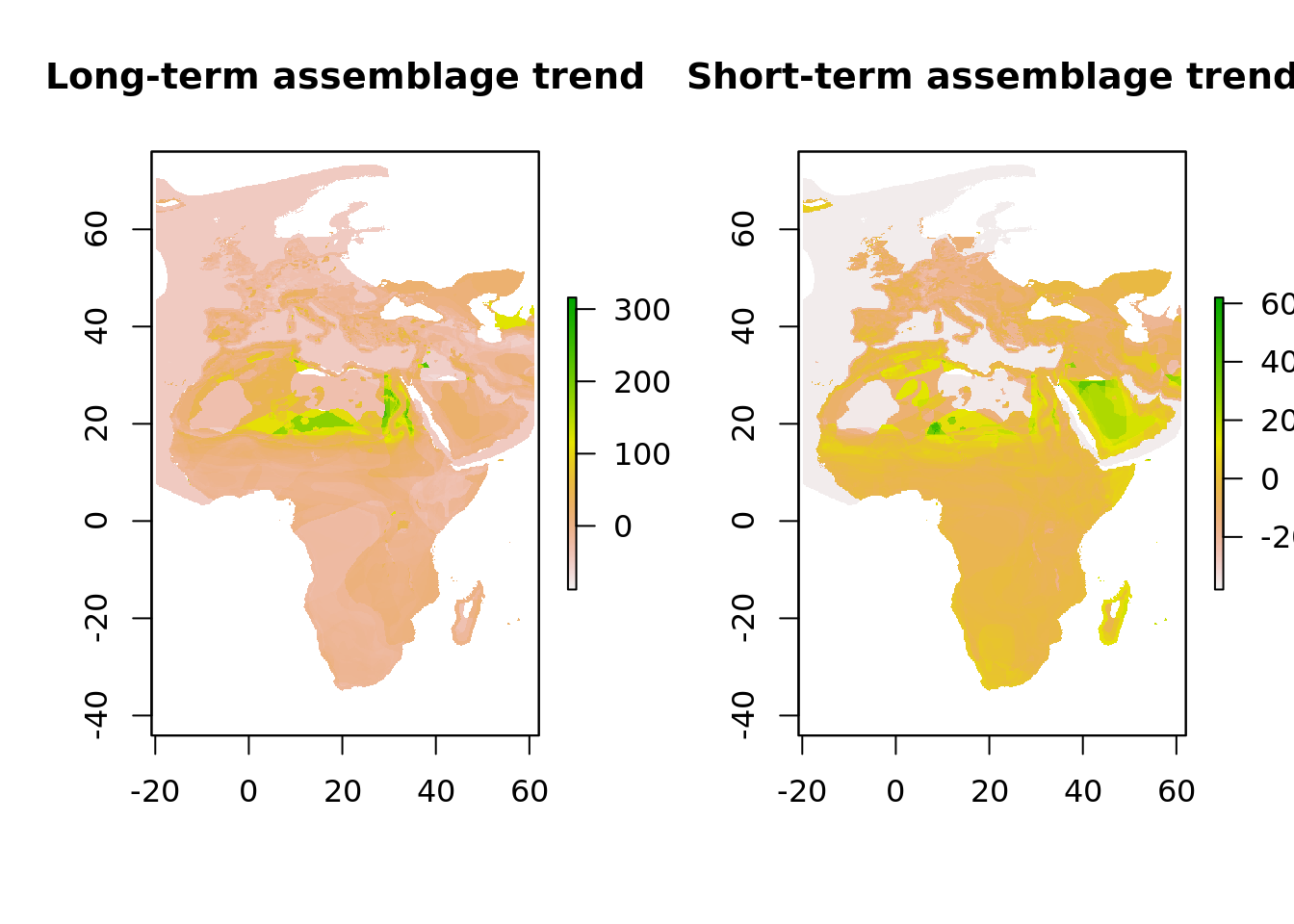 And a similar plot for the number of species that the assemblages consist of.
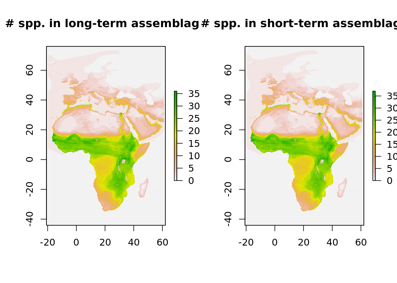
par(mfrow = c(1, 2))
plot(trend_long_counts, main = "# spp. in long-term assemblage")
plot(trend_short_counts, main = "# spp. in short-term assemblage")