2 Simple rain segmentation
Classifying rain using RHOHV and DPR (depolarization ratio, Kilambi et al.) gets us most of the way for an elegant filtering procedure for rain, but the issue remains on the edges of rain clouds, where these dual-pol products or derivatives are less performant. Here, we try an image processing technique that can help improve the rain segmentation a bit further.
2.1 Problem
Let’s load a pvol with rain and show what it looks like after range-bias correction.
pvolfile <- "data/20201002/NLHRW_pvol_20201002T1205_6356.h5"
pvol <- read_pvolfile(file = pvolfile, param = "all")
vp <- calculate_vp(pvolfile, verbose = FALSE)
ppi_rainy <- integrate_to_ppi(pvol, vp, xlim = c(-180000, 180000), ylim = c(-180000, 180000), res = 500, param = "DBZH")
plot(ppi_rainy)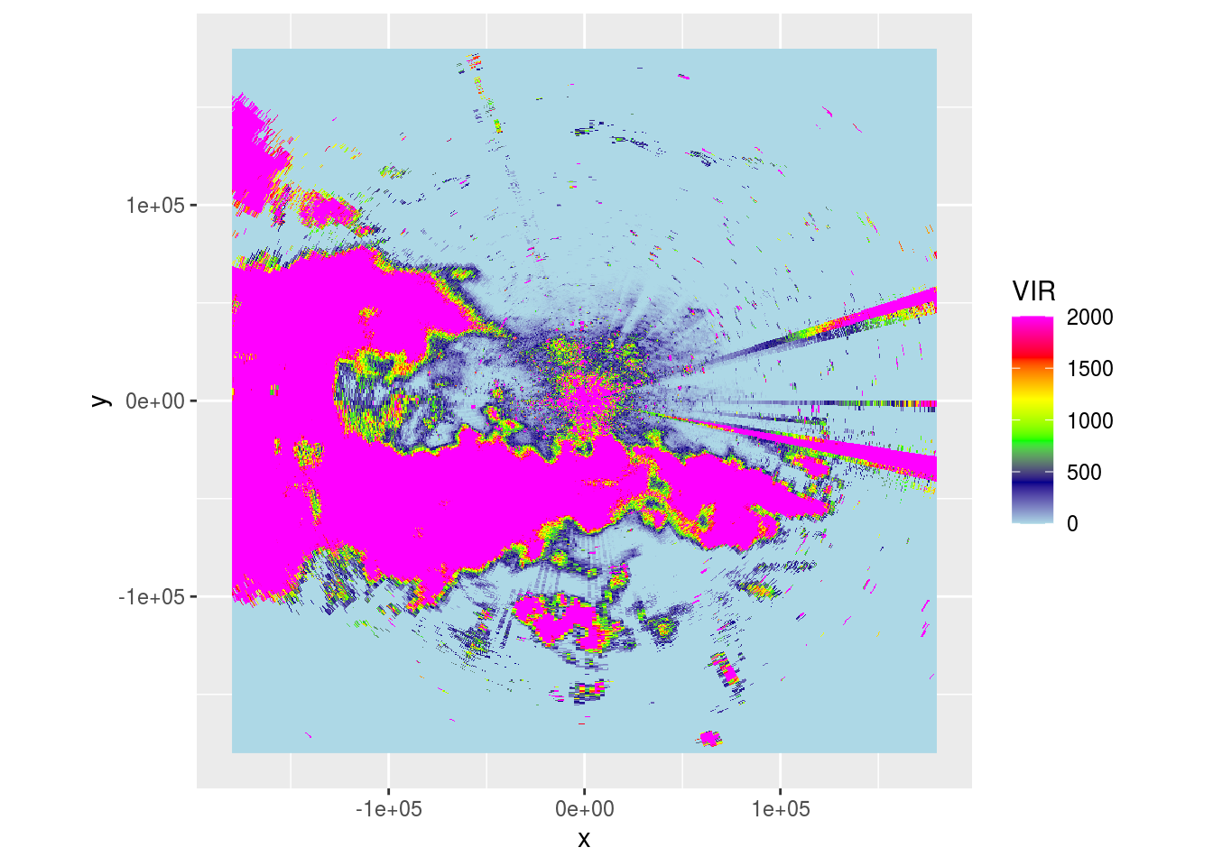
2.2 Solution
There’s clearly a lot of rain in this scan. Now, we can filter this using the depolarization ratio, but that requires some additional steps:
- For some reasons not all radar rangegates have the full combination of
DBZH,DBZVandRHOHVcontained within, which means that for these pixels either theZDRcannot be calculated, orRHOHVis not available for the calculation of theDPR. - The edges of rain clouds are not necessarily well identified by the
DPR(orRHOHVfor that matter), so we need to apply some buffering/smoothing to improve this.
2.2.1 Filter pixels without dual-pol measurements
First, let’s make a plot of what pixels we lose if we filter for pixels where we can calculate the DPR for, which means both DBZV and RHOHV must have been available.
pvol_original <- pvol  # Let's keep the original pvol for comparison

pvol <- calculate_param(pvol,
                        ZDRL = 10 ** ((DBZH - DBZV) /10),
                        DPR = 10 * log10((ZDRL + 1 - 2 * ZDRL^0.5 * RHOHV) / (ZDRL + 1 + 2 * ZDRL^ 0.5 * RHOHV)),
                        DBZHO = DBZH)

pvol$scans <- lapply(pvol$scans, function(x) {
  x$params[["DBZH"]][is.na(x$params[["DPR"]])] <- NA
  x$params[["RHOHV"]][is.na(x$params[["DBZH"]])] <- NA
  return(x)
})

ppiplot_rainy <- plot(ppi_rainy) + ggtitle("Original RBC PPI")
ppi_dualpol <- integrate_to_ppi(pvol, vp, xlim = c(-180000, 180000), ylim = c(-180000, 180000), res = 500, param = "DBZH")
ppiplot_dualpol <- plot(ppi_dualpol) + ggtitle("Dual-pol available RBC PPI")

ppiplot_rainy + ppiplot_dualpol + plot_layout(guides = "collect")
We can also plot the difference, for which we make a difference of 0 transparent to better see where the PPI pixels are changed most dramatically, and we plot the differences in a histogram.
ppi_difference <- ppi_dualpol
ppi_difference$data$VIR <- ppi_rainy$data$VIR - ppi_dualpol$data$VIR
ppi_difference$data$VIR[ppi_difference$data$VIR == 0] <- NA

ppiplot_difference <- plot(ppi_difference) +
  scale_fill_viridis_c(trans = "log10") +
  labs(fill = "VIR diff") +
  # guides(fill = guide_legend(title = "VIR diff")) +
  ggtitle("Original pixels - pixels with DPR")

as.data.frame(ppi_difference$data) %>%
  drop_na() %>%
  filter(VIR < 1e5) %>%
  ggplot() +
  geom_histogram(aes(x = VIR)) +
  scale_x_continuous(trans = "log10") +
  labs(x = "VIR diff") -> plot_difference

ppiplot_difference + plot_difference
The PPI and histogram suggest most VIR differences occur in regions with already high reflectivities, which in this particular PPI must have been mostly rain. So filtering these pixels doesn’t hurt much. Presumably this applies across the board, but that’ll require some further investigation. Nevertheless, for now we assume filtering pixels for the presence of DBZH seems reasonable.
2.2.2 Image processing
We start by illustrating the approach to a single scan. We use the DPR as the main masking methodology, though it’s possible to extend this technique to include RHOHV, as a combined approach may perform better. We plot a \((r,a)\) plot where white pixels are classified as rain (dpr < -12), and black pixels are not.
scan.dpr <- as.cimg(pvol$scans[[1]]$params[["DPR"]])

(scan.dpr <= -12 & !is.na(scan.dpr)) %>%
  plot()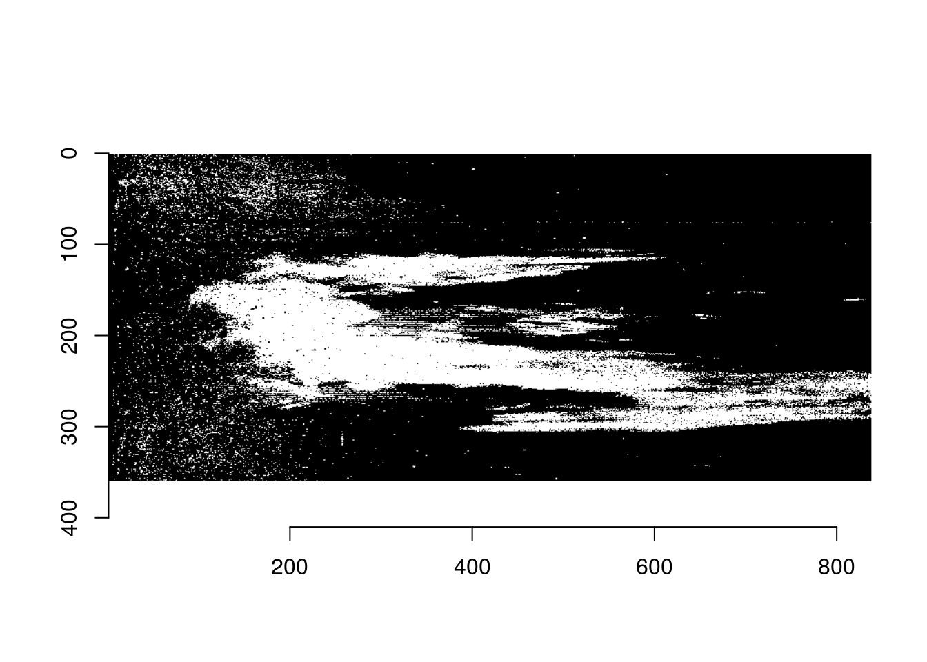
This shows a lot of pixels, especially close to the radar (lower x-values), get flagged as rain because of the DPR value. This is why Kilambi et al. recommend despeckling. Let’s use a median-filter to apply this despeckling.
(scan.dpr <= -12 & !is.na(scan.dpr)) %>%
  medianblur(4) %>%
  threshold(0) ->
  despeckled

despeckled %>% plot()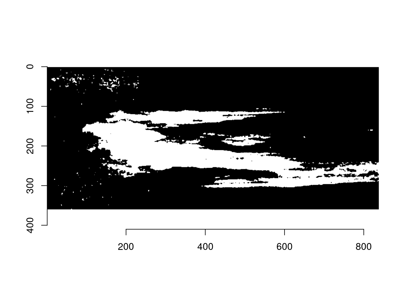
That already looks better, but now we have ‘blurred’ out some of the regions to larger pixels. If we assume that true rain occurs mostly in larger areas, we can compute the contiguous areas which are flagged as precipitation, calculate the surface (number of pixels within) and filter based on a minimum number of pixels. In this case, we classify rain only as rain if it covers at least 50 pixels/rangegates.
despeckled %>%
  split_connected() %>%
  purrr::keep(~ sum(.) > 50) %>%
  parany() -> areafilter

areafilter %>% plot()
Now, there’s a chance we miss some pixels left and right, so if we conservatively filter out rain, we could buffer these areas a bit. So, we’ll calculate the euclidean distance from non-rain to rain pixels and if that distance is < 5 units, we’ll flag these pixels as rain as well.
areafilter %>%
  distance_transform(1, metric = 2) %>%
  threshold(5) -> buffered

(-buffered) %>%
  plot()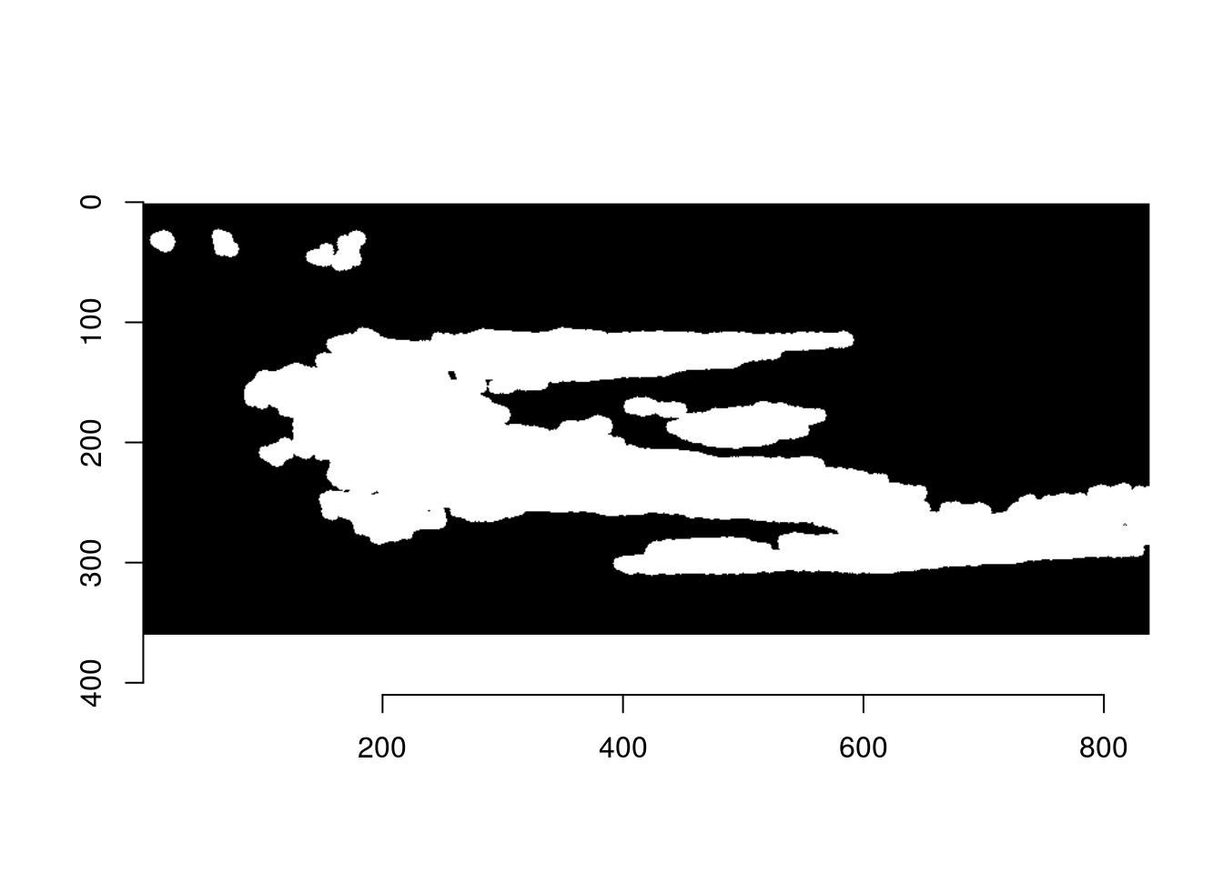
We can now check what it looks like if we apply this masking approach to the scans and polar volumes. First we plot the single scan we’ve cleaned so far.
pvol_buffer <- pvol
pvol_thresh <- pvol

pvol_buffer$scans[[1]]$params$DBZH[!as.matrix(buffered)] <- NA
pvol_thresh$scans[[1]]$params$DBZH[pvol_thresh$scans[[1]]$params$DPR < -12 | pvol_thresh$scans[[1]]$params$RHOHV >= 0.95] <- NA

(plot(pvol_original$scans[[1]], xlim = c(0, 180000)) + ggtitle("Original PVOL")) /
  (plot(pvol_thresh$scans[[1]], xlim = c(0, 180000)) + ggtitle("Simple threshold filter")) /
  (plot(pvol_buffer$scans[[1]], xlim = c(0, 180000)) + ggtitle("Buffered threshold filter"))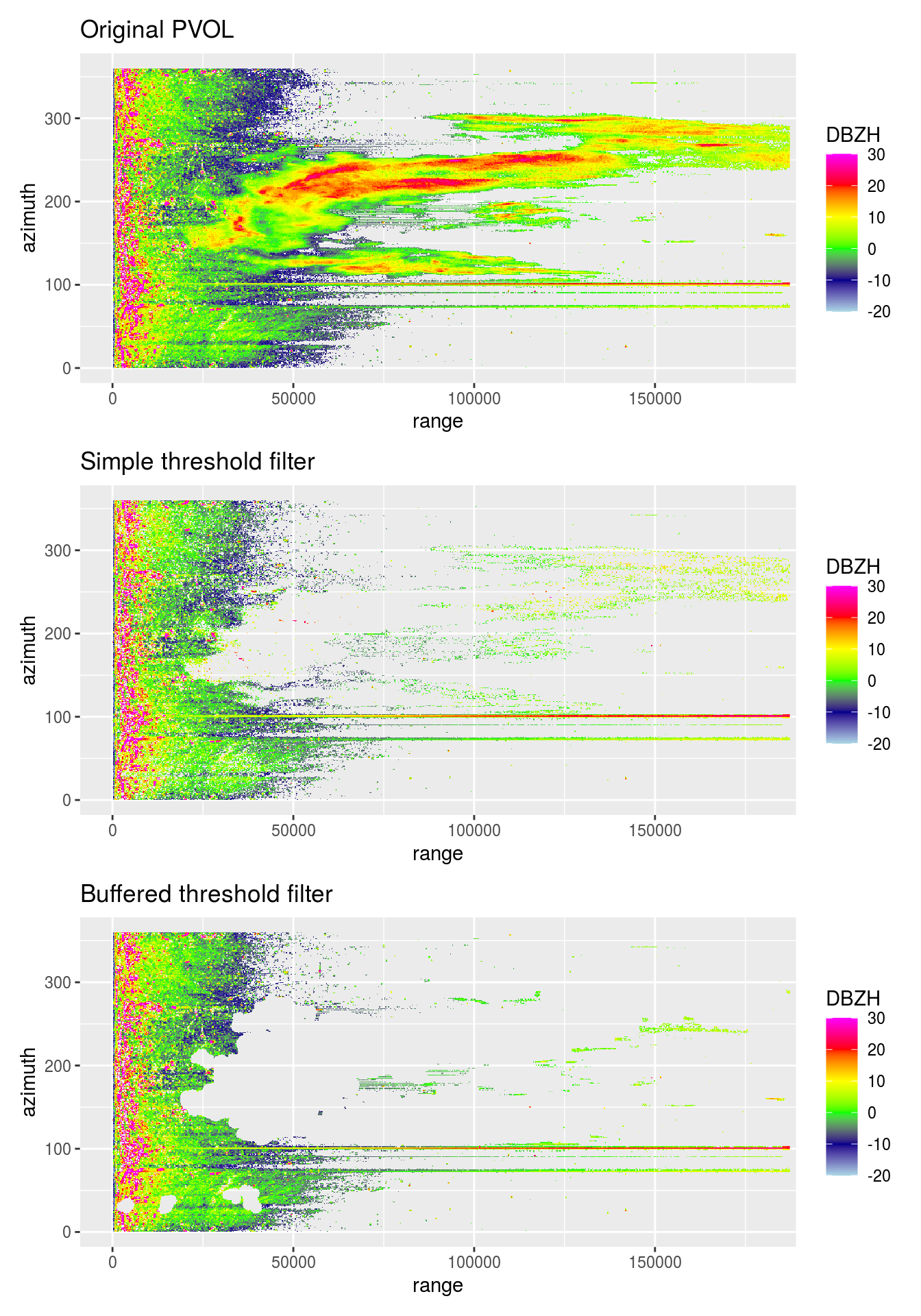
Except for the continuing presence of some interference pattern, and possibly filtering out some areas with ground clutter or wind parks, we see a much cleaner rain filtering than before in the buffered threshold filter.
Now let’s apply it to the full pvol.
rainfilter <- function(scan) {
  if (scan$geo$elangle < 90) {
    dpr <- as.cimg(scan$params[["DPR"]])
    (dpr <= -12 & !is.na(dpr)) %>%
      medianblur(4) %>%  # Works adequate for de-speckling
      threshold(0) %>%  # Set all pixels that have been affected by median blurring to 1, rest to 0
      split_connected() %>%  # Split image in contiguous areas classified as rain
      purrr::keep(~ sum(.) > 50) %>%  # Only keep contiguous rain areas if area is > 50 pixels
      parany() -> contiguous  # Merge to 1 image again
    if (!is.null(contiguous)) {  # Only buffer if any rain areas of > 50 pixels are retained
      contiguous %>%
        distance_transform(1, 2) %>%  # Calculate Euclidean distance (2nd argument) to pixels classified as 1
        threshold(5) -> dpr_filter

      dpr_filter <- -dpr_filter
      scan$params$DBZH[!as.matrix(dpr_filter)] <- NA
    }
  }
  return(scan)
}

pvol$scans <- lapply(pvol$scans, function(x) {
  x$params[["DBZH"]][is.na(x$params[["DPR"]])] <- NA
  # x$params[["DBZH"]][x$params[["RHOHV"]] >= 0.95] <- NA
  # x$params[["DBZH"]][x$params[["DPR"]] < -12] <- NA
  x <- rainfilter(x)
  return(x)
})
And once again, calculate RBC and plot the resulting PPI.
ppi_buffered <- integrate_to_ppi(pvol, vp, xlim = c(-180000, 180000), ylim = c(-180000, 180000), res = 500, param = "DBZH")
ppiplot_buffered <- plot(ppi_buffered) + ggtitle("Buffered rain filtering")

(ppiplot_rainy + ggtitle("Original RBC PPI")) + ppiplot_buffered + plot_layout(guides = "collect")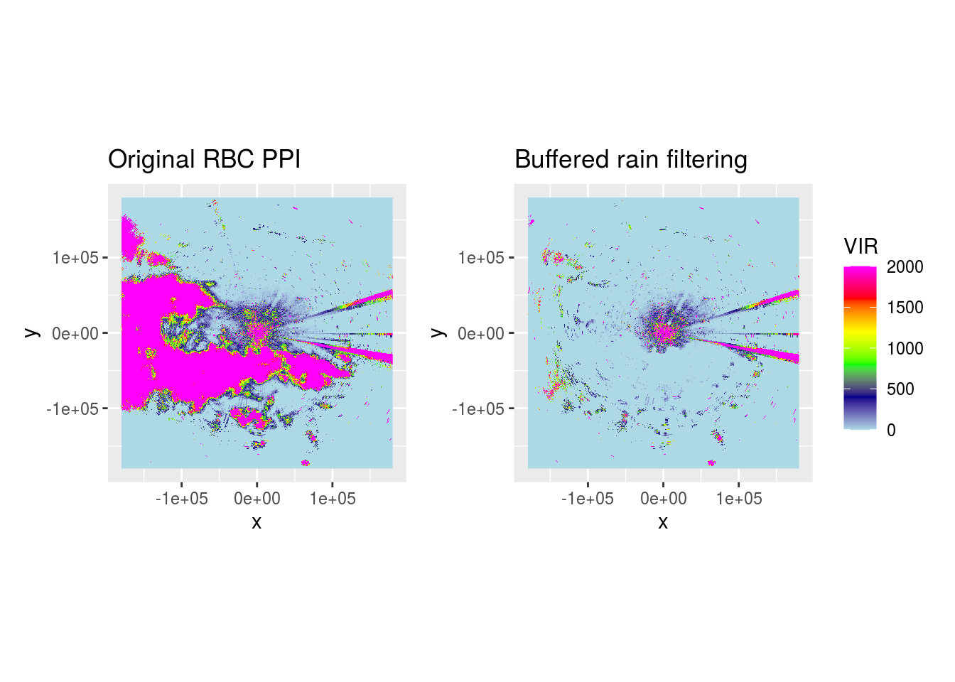
At first sight the RBC PPI may look quite messy after filtering, but overall this approach seems to work quite well:
- Most of the edges of rain clouds are removed quite well, with mostly the exception of those at > 80km from the radar, but this is probably mostly due to dual-pol measurements not working well anymore at these distances anyways.
- We can still apply post-processing to the RBC PPIs, for example by filtering out pixels which have too high values of
VIRfor them to be birds. Or to simply despeckle, or calculate a median value across the whole image. - We have now applied a single buffering procedure to all the scans at all elevations, but this could possibly be tweaked further for each elevation. At higher elevations, we can probably filter quite agressively, and especially if we also include altitude above the ground in our filtering approach.
- Many of the speckles that are visible are not necessarily rain, but were already present in the original RBC PPI, so this approach definitely did not worsen this issue much.
- Finally, as the outcome of the range-bias correction is a projection of the integrated reflections on a cartesian grid, we could consider to vertically stack all rain segmentations after projecting them from slant to ground range and then using this combined mask to filter out the entire regions covered by rain. This assumes rain clouds always stretch vertically along the full altitude range covered by the radar, which may not be realistic, but to create a clean and interpretable RBC PPI this could be an acceptable trade-off.